Assignment 4-RADIOSS Material Laws Challenge

ASSIGNMENT 4 - RUPTURE PLATE

CASE 1

Objective:

The main objective here is to run the model as it is without changing any values and saving it with the name Law2_epsmax_failure than creating Energy graphs & Rigid wall curves and observe how the transformation is going on.

Procedure:

• First download the .rad file from the challenge question page
• Than Go to File - Import - Solverdeck - Select the file from the location where it is saved -Click on Import
• After Importing go to model tab and check all the values than
• Rename the card to Law2_epsmax_failure
• Now Go to Analysis - Radioss - Select the location where the files should be saved
• Keep Export options:all , Run options: analysis , run number: 1 , Options : -nt 4
• Than hit on Radioss option it starts simulation of the file
• Now we will be getting a Out file as shown below open this in notepad

• After a certain time the simulation running will stop than go through those and there Total no. of cycles , Energy error & Mass error , Total starter run time , engine run time all these values can be taken from there.
• After observing all these values note those values properly.

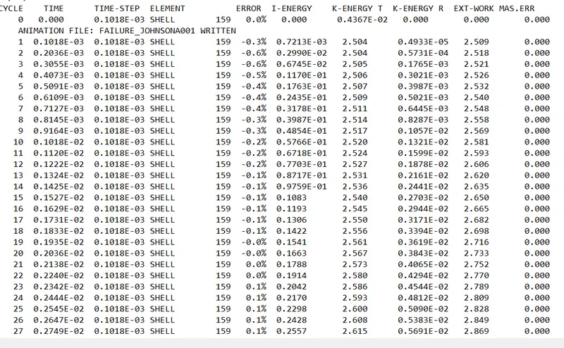
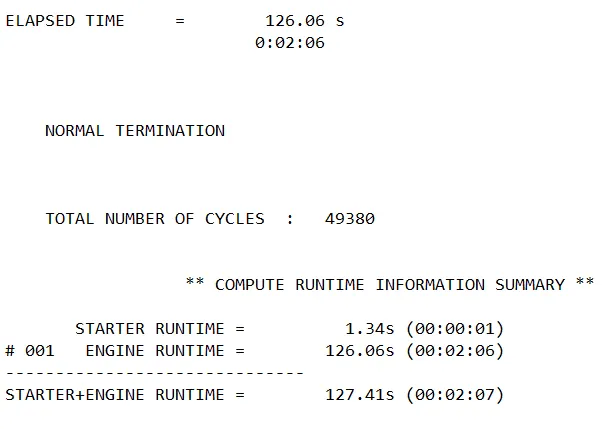
From above we can know,

Total no. of cycles = 49380

Elapsed time = 126.06 sec

Max. Positive energy error = +1.3%

Min . Negative ernergy error = -0.3%

Mass error. = 0.000

• From this we can get to know that the positive energy is less than 2% which is accceptable incase of QEPH & Fully integrated element properties and also Min energy error is always acceptable as it means the amount of energy which is dissipated.
• Here coming to Mass error it is 0 as here no mass is added to meet specified time step.
• Than select a Multi page option and in new page selct Hyperview.
• Select the .h3d files for case 1 worked and import that in Hyperview window
• After importing there will be a Ball and circular plate type model present on the screen
• Start working on the model
• Switch on the mesh using shaded elements & meshlines option
• Than by using contour option vonmises stress is applied & indicated on the model and by using animation option we can test how the crash is happening & how is it failing can be anlysed.

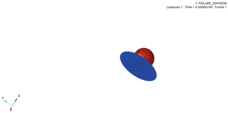
Before Failing

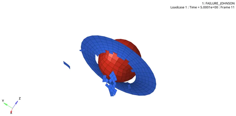
After Failing

• Animation can be recorded by User interface record option as below-

• From Case 1 animation we can get to know that failing occurs directly by getting elements deleted & in this way breaking occurs.
• Next by using hypergraphs 2D plot the Energy graphs and Rigid wall forces as
• Go to hypergraphs - Select the T01 file to plot the graphs than-
• Select X type - Time & Y type - Global variable - Select the type of energies to be plotted on the graph -than select MAG - Click on Apply.
• Here we will select Internal energy, Kinetic energy , Contact energy , total energy, hourglass energy etc...than the graph will be plotted.

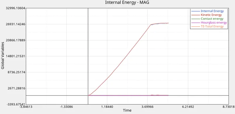
• By this Energy graphs we can get to know that the Hourglass energy & contact energy are lying near the origin as it is ok because always these both values should be less so it passes with this statement
• Here as initially the IE , KE , & Total energy are low gradually when the object strikes other the graph starts increasing its growth but after certain continuous increase it stops and maintains neutrally and comes to rest.
• Now start the new plot by going to File - New - Plot - The new hypergraphs page will be created
• Than here in X type select as Time and Y type as Rigid wall - 1 Punch - Than select Fx , Fy , Fz , Total forces , Total resultant forces etc.. should be plotted on the graph.

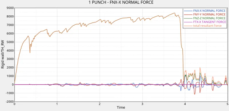
• By this RW graph we can observe that FNzz Normal force & total resultant force are increasing gradually and goes very high upto some extent and starts drowning when it is nearby to rest but other all forces will be lying near the X axis line.

Conclusion:

By performing whole procedure in step by step manner we will get to know the energy values , rigid wall force values indicated graphically and also Energy error & mass error , Total no. of cycles , Time step , Total elapsed time .....these all values can be known and this will be used for next case to know consequences after certain changes.

CASE 2

Objective:

The main objective here is to run the model as it is but changing some values in Failure card and saving it with the name Law2_epsmax_Crack which is simulated than creating Energy graphs & Rigid wall curves and observe how the transformation is going on.

Given,

Ifail_sh = 1

Dadv = 1

Ixfem = 1

Procedure:

• Here .Rad file will be taken from previous case out file as -
• Go to File - Import - Solverdeck - Select the previous Case 1 file from the location where it is saved- from that select .001 rad file -Click on Import
• After Importing go to model tab and check all the values than
• Rename the card to Law2_epsmax_Crack
• Than Go to Failures card - In the Failure card change the values of Ifail_sh = 1, Dadv =1 , & Ixfem = 1
• Now Go to Analysis - Radioss - Select the location where the files should be saved
• Keep Export options:all , Run options: analysis , run number: 1 , Options : -nt 4
• Than hit on Radioss option it starts simulation of the file
• Now we will be getting a Out file as shown below open this in notepad

• After a certain time the simulation running will stop than go through those and there Total no. of cycles , Energy error & Mass error , Total starter run time , engine run time all these values can be taken from there.
• After observing all these values note those values properly.

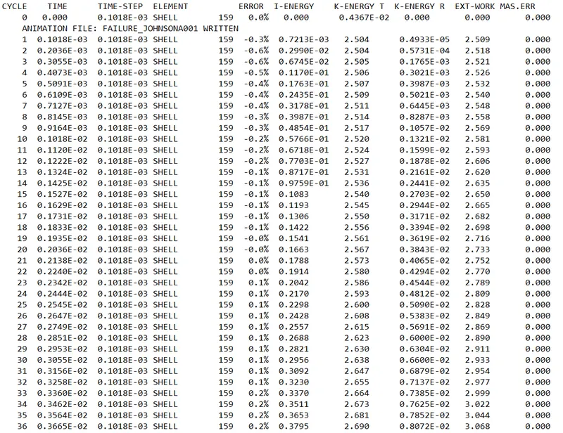
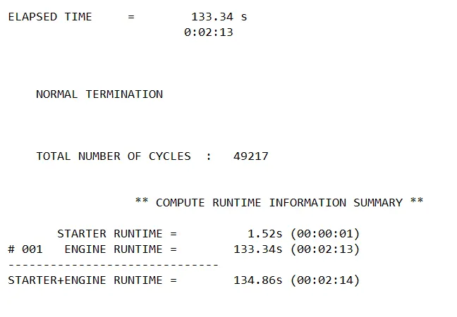
From above we can know,

Total no. of cycles = 49217

Elapsed time = 133.34 sec

Max. Positive energy error = +4.5%

Min . Negative ernergy error = -0.3%

Mass error. = 0.000

• From this we can get to know that the positive energy is more than 2% which is not accceptable incase of QEPH & Fully integrated element properties and also Min energy error is always acceptable as it means the amount of energy which is dissipated.
• Here coming to Mass error it is 0 as here no mass is added to meet specified time step.
• Than select a Multi page option and in new page selct Hyperview.
• Select the .h3d files for case 2 worked and import that in Hyperview window
• After importing there will be a Ball and circular plate type model present on the screen
• Start working on the model
• Switch on the mesh using shaded elements & meshlines option
• Than by using contour option vonmises stress is applied & indicated on the model and by using animation option we can test how the crash is happening & how is it failing can be anlysed.

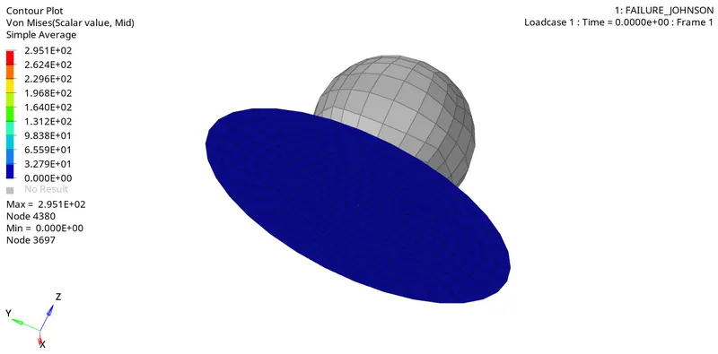
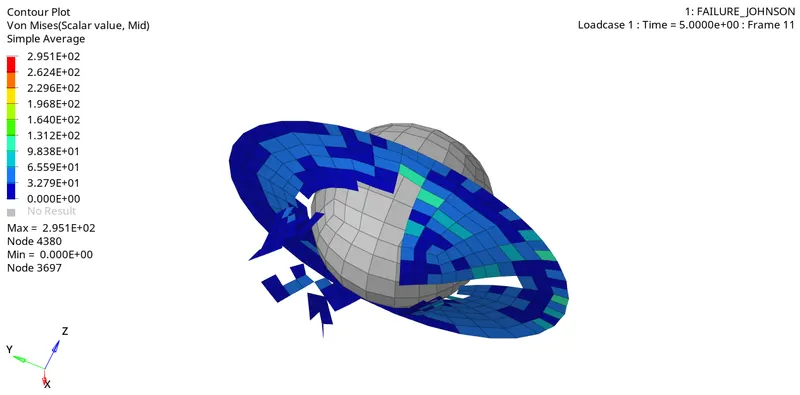
• After this animation we get to know that the model will be failing very rapidly as it is a failure model due to high energy error and so..it may also affect the model
• Next by using hypergraphs 2D plot the Energy graphs and Rigid wall forces as
• Go to hypergraphs - Select the T01 file to plot the graphs than-
• Select X type - Time & Y type - Global variable - Select the type of energies to be plotted on the graph -than select MAG - Click on Apply.
• Here we will select Internal energy, Kinetic energy , Contact energy , total energy, hourglass energy etc...than the graph will be plotted.

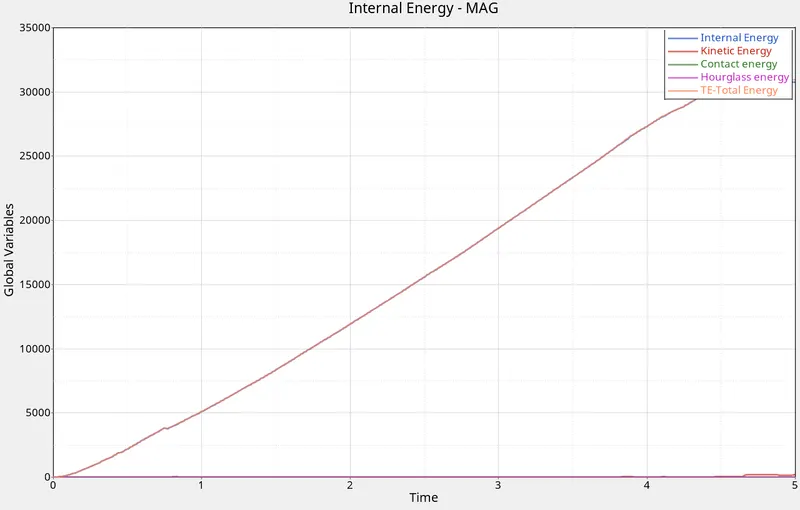
• From this energy graph we can observe that Total energy & Internal energies graph is gradually increasing and all other energies like KE , Contact & Hourglass energy are near the X axis line .
• Next we will be plotting graphs for Rwall forces as -
• Start the new plot by going to File - New - Plot - The new hypergraphs page will be created
• Than here in X type select as Time and Y type as Rigid wall - 1 Punch - Than select Fx , Fy , Fz , Total forces , Total resultant forces etc.. should be plotted on the graph.

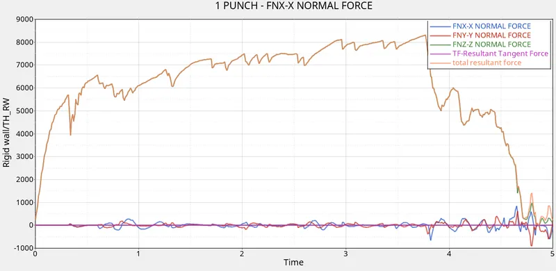
• By this RW graph we can observe that FNzz Normal force & total resultant force are increasing gradually and goes very high upto some extent and starts drowning when it is nearby to rest but other all forces will be lying near the X axis line.

Conclusion:

By performing whole procedure in step by step manner we will get to know the energy values , rigid wall force values indicated graphically and also Energy error & mass error , Total no. of cycles , Time step , Total elapsed time .....these all values can be known and .Rad file of this case will be used for next case to know consequences after certain changes.

CASE 3

Objective:

The main objective in Case 3 is to run the model as it is without changing any values directly delete the Failure johnson card and save it with the name Law2_epsmax_nofail than creating Energy graphs & Rigid wall curves and observe how the transformation is going on.

Procedure:

• Here .Rad file will be taken from previous case out file as -
• Go to File - Import - Solverdeck - Select the previous Case 2 file from the location where it is saved- from that select .001 rad file -Click on Import
• After Importing go to model tab and check all the values than
• Rename the card to Law2_epsmax_nofail
• Than Go to Failures card - Delete the failure card directly which contains these values Ifail_sh = 1, Dadv =1 , & Ixfem = 1
• Now Go to Analysis - Radioss - Select the location where the files should be saved
• Keep Export options:all , Run options: analysis , run number: 1 , Options : -nt 4
• Than hit on Radioss option it starts simulation of the file
• Now we will be getting a Out file as shown below open this in notepad

• After a certain time the simulation running will stop than go through those and there Total no. of cycles , Energy error & Mass error , Total starter run time , engine run time all these values can be taken from there.
• After observing all these values note those values properly.

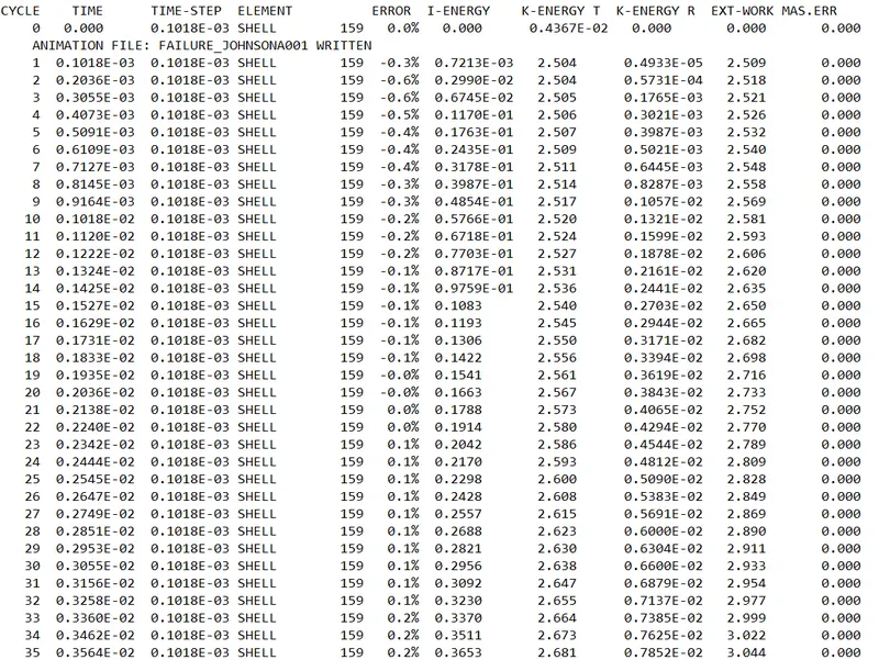
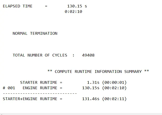
From above we can know,

Total no. of cycles = 49408

Elapsed time = 130.15sec

Max. Positive energy error = +1.5%

Min . Negative ernergy error = -0.1%

Mass error. = 0.000

• From this we can get to know that the positive energy is less than 2% which is accceptable incase of QEPH & Fully integrated element properties and also Min energy error is always acceptable as it means the amount of energy which is dissipated.
• Here coming to Mass error it is 0 as here no mass is added to meet specified time step.
• Than select a Multi page option and in new page selct Hyperview.
• Select the .h3d files for case 3 worked and import that in Hyperview window
• After importing there will be a Ball and circular plate type model present on the screen
• Start working on the model
• Switch on the mesh using shaded elements & meshlines option
• Than by using contour option vonmises stress is applied & indicated on the model and by using animation option we can test how the crash is happening & how is it failing can be anlysed.

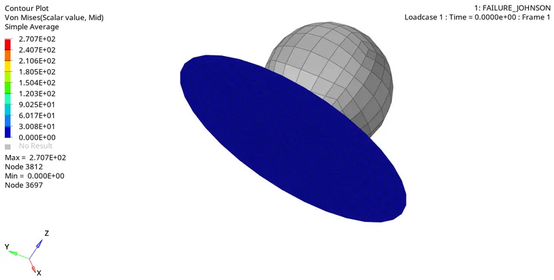
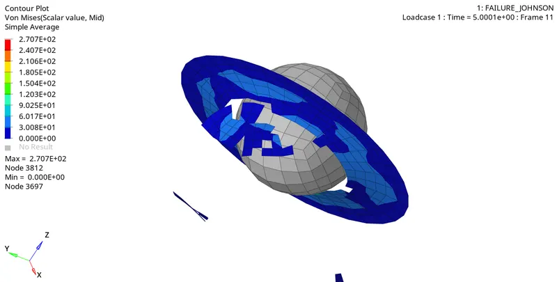
• After this animation we get to know that the model will be failing as it is not a failure model because of no failure card which will be reflected while this .rad file used in the next case
• Next by using hypergraphs 2D plot the Energy graphs and Rigid wall forces as
• Go to hypergraphs - Select the T01 file to plot the graphs than-
• Select X type - Time & Y type - Global variable - Select the type of energies to be plotted on the graph -than select MAG - Click on Apply.
• Here we will select Internal energy, Kinetic energy , Contact energy , total energy, hourglass energy etc...than the graph will be plotted.

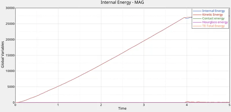
• This Energy graph is in a controlled way as there is no failure card in this
• From this energy graph we can observe that Only Total energy & Internal energies graph is gradually increasing and all other energies like KE , Contact & Hourglass energy are near the X axis line .
• Next we will be plotting graphs for Rwall forces as -
• Start the new plot by going to File - New - Plot - The new hypergraphs page will be created
• Than here in X type select as Time and Y type as Rigid wall - 1 Punch - Than select Fx , Fy , Fz , Total forces , Total resultant forces etc.. should be plotted on the graph.

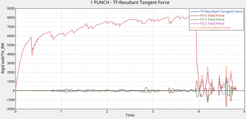
• By this RW graph we can observe that Total Force in Fzz & total resultant force are increasing gradually and goes very high upto some extent and starts drowning when it is nearby to rest but other all forces will be lying near the X axis line.

Conclusion:

By performing whole procedure in step by step manner we will get to know the energy values , rigid wall force values indicated graphically and also Energy error & mass error , Total no. of cycles , Time step , Total elapsed time .....these all values can be known and .Rad file of this case will be used for next case to know consequences after certain changes.

CASE 4

Objective:

The main objective in Case 4 is to run the model as it is without changing any values but directly delete the value of EPS_p_max and save it with the name Law2 than creating Energy graphs & Rigid wall curves and observe how the transformation is going on.

Procedure:

• Here .Rad file will be taken from previous case out file as -
• Go to File - Import - Solverdeck - Select the previous Case 3 file from the location where it is saved- from that select .001 rad file -Click on Import
• After Importing go to model tab and check all the values than
• Rename the card to Law2
• Than Go to - Mterials - Aluminium - In the dropdown there will be values of E , n , b , Nu etc...from this delete Eps_P_max value and make it to 'Zero' as shown below-

• Now Go to Analysis - Radioss - Select the location where the files should be saved
• Keep Export options:all , Run options: analysis , run number: 1 , Options : -nt 4
• Than hit on Radioss option it starts simulation of the file
• Now we will be getting a Out file as shown below open this in notepad

• After a certain time the simulation running will stop than go through those and there Total no. of cycles , Energy error & Mass error , Total starter run time , engine run time all these values can be taken from there.
• After observing all these values note those values properly.

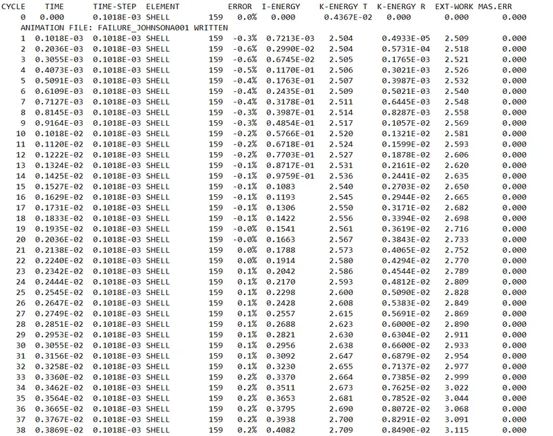
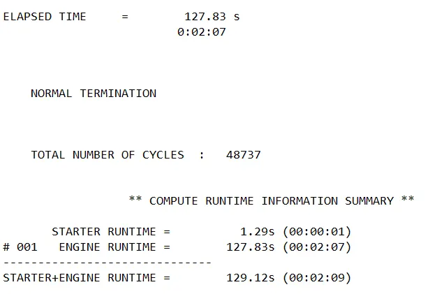
From above we can know,

Total no. of cycles = 48737

Elapsed time = 127.83 sec

Max. Positive energy error = +3%

Min . Negative ernergy error = -0.1%

Mass error. = 0.000

• From this we can get to know that the positive energy is more than 2% which is not so accceptable incase of QEPH & Fully integrated element properties and also Min energy error is always acceptable as it means the amount of energy which is dissipated.
• Here coming to Mass error it is 0 as here no mass is added to meet specified time step.
• Than select a Multi page option and in new page selct Hyperview.
• Select the .h3d files for case 3 worked and import that in Hyperview window
• After importing there will be a Ball and circular plate type model present on the screen
• Start working on the model
• Switch on the mesh using shaded elements & meshlines option
• Than by using contour option vonmises stress is applied & indicated on the model and by using animation option we can test how the crash is happening & how is it failing can be anlysed.

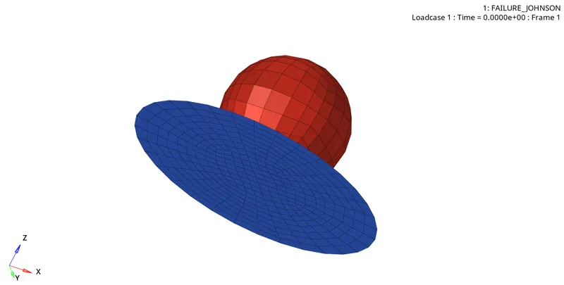
BEFORE FAILING

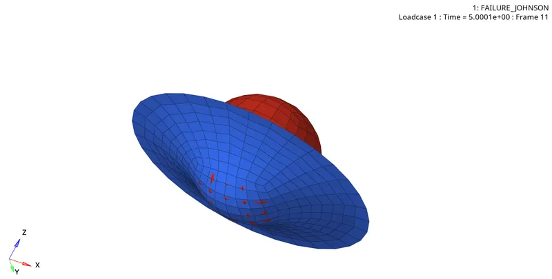
AFTER FAILING

AFTER FAILING SHOWN THROUGH VONMISES STRESS

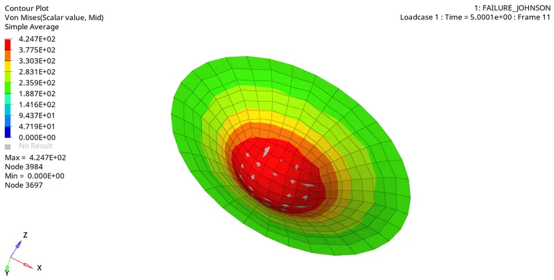
• As here we have used the .rad file of previous no failure card model here the failure will be happenig only by crackng of elements i.e...here the elements will be not totally deleting.
• Next by using hypergraphs 2D plot the Energy graphs and Rigid wall forces as
• Than Go to hypergraphs - Select the T01 file to plot the graphs than-
• Select X type - Time & Y type - Global variable - Select the type of energies to be plotted on the graph -than select MAG - Click on Apply.
• Here we will select Internal energy, Kinetic energy , Contact energy , total energy, hourglass energy etc...than the graph will be plotted.

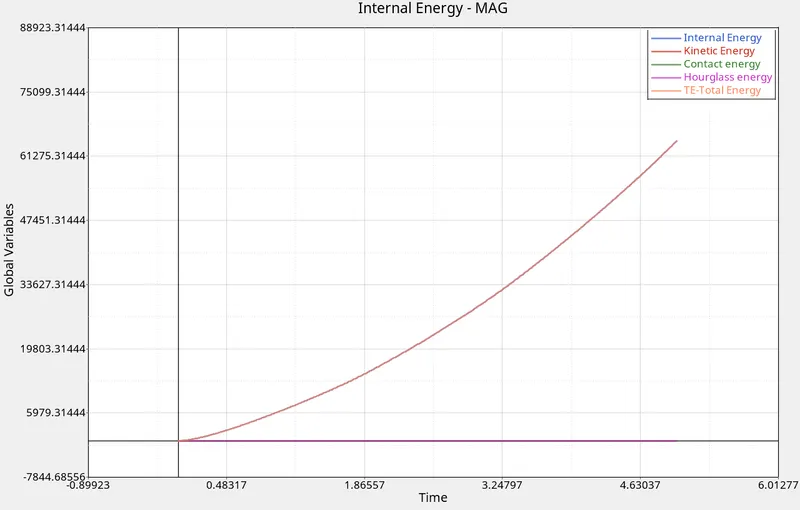
• This Energy graph is in a controlled way as this is the .rad file of no failure card model .
• From this energy graph we can observe that Only Total energy & Internal energies graph is slowly & progressively increasing and all other energies like KE , Contact & Hourglass energy are near the X axis line .
• Next we will be plotting graphs for Rwall forces as -
• Start the new plot by going to File - New - Plot - The new hypergraphs page will be created
• Than here in X type select as Time and Y type as Rigid wall - 1 Punch - Than select Fx , Fy , Fz , Total forces , Total resultant forces etc.. should be plotted on the graph.

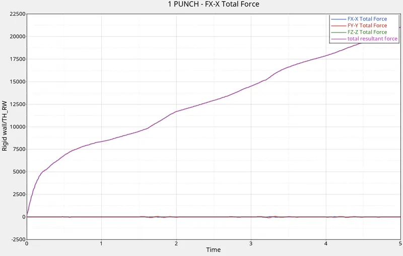
• By this RW graph we can observe that Total Force in Fzz & total resultant force are increasing gradually and properly and goes very high upto some extent and stops but other all forces will be lying near the X axis line with very clean representation with very even lines.

Conclusion:

By performing whole procedure in step by step manner we will get to know the energy values , rigid wall force values indicated graphically and also Energy error & mass error , Total no. of cycles , Time step , Total elapsed time .....these all values can be known and .Rad file of this case will be used for next case to know consequences after certain changes.

CASE 5

Objective:

The main objective in Case 5 is to run the model by changing material model to Law 1 Elastic save it with the name Law1 with same E , n , Nu Rho etc.. values & than creating Energy graphs & Rigid wall curves and observe how the transformation is going on.

Procedure:

• Here .Rad file will be taken from previous case out file as -
• Go to File - Import - Solverdeck - Select the previous Case 4 file from the location where it is saved- from that select .001 rad file -Click on Import
• After Importing go to model tab and check all the values than
• Rename the card to Law1
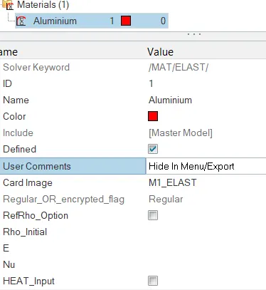
• Here we will be changingCard image from M2_Plas_Johns_Zeril to M1_Elast.
• After this update with same E , Rho , Nu values as before in this M1_Elast card image dropdown

• Now Go to Analysis - Radioss - Select the location where the files should be saved
• Keep Export options:all , Run options: analysis , run number: 1 , Options : -nt 4
• Than hit on Radioss option it starts simulation of the file
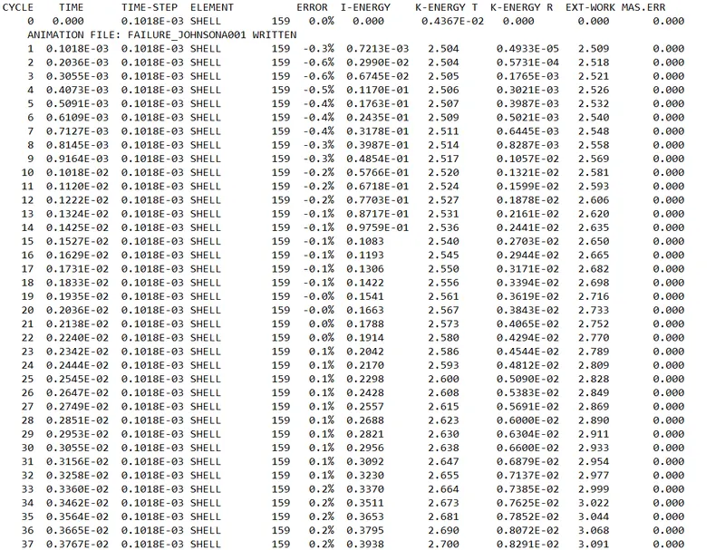
• Now we will be getting a Out file as shown below open this in notepad

• After a certain time the simulation running will stop than go through those and there Total no. of cycles , Energy error & Mass error , Total starter run time , engine run time all these values can be taken from there.
• After observing all these values note those values properly.

From above we can know,

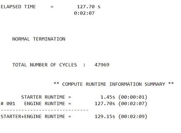
Total no. of cycles = 47969

Elapsed time = 127.70 sec

Max. Positive energy error = +4%

Min . Negative ernergy error = -0.1%

Mass error. = 0.000

• From this we can get to know that the positive energy is more than 2% which is not so accceptable incase of QEPH & Fully integrated element properties and also Min energy error is always acceptable as it means the amount of energy which is dissipated.
• Here coming to Mass error it is 0 as here no mass is added to meet specified time step.
• Than select a Multi page option and in new page selct Hyperview.
• Select the .h3d files for case 5 worked and import that in Hyperview window
• After importing there will be a Ball and circular plate type model present on the screen
• Start working on the model
• Switch on the mesh using shaded elements & meshlines option
• Than by using contour option vonmises stress is applied & indicated on the model and by using animation option we can test how the crash is happening & how is it failing can be anlysed.

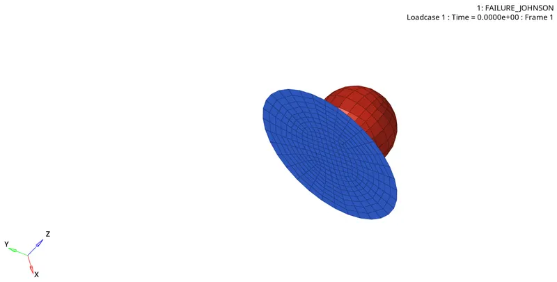
BEFORE FAILING

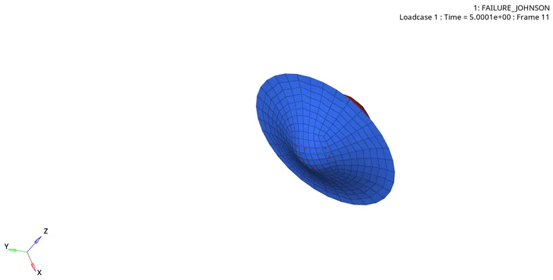
AFTER FAILING

AFTER FAILING SHOWN THROUGH VONMISES STRESS

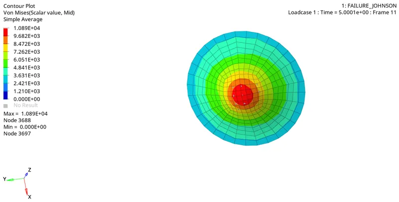
• As here we have used the .rad file of previous file isused and with Material model E1_Elast is used as this means it is a elastic model there is very less chance of elements deleting here the elements will be not totally deleted rather those are slightly cracked.
• Next by using hypergraphs 2D plot the Energy graphs and Rigid wall forces as
• Go to hypergraphs - Select the T01 file to plot the graphs than-
• Select X type - Time & Y type - Global variable - Select the type of energies to be plotted on the graph -than select MAG - Click on Apply.
• Here we will select Internal energy, Kinetic energy , Contact energy , total energy, hourglass energy etc...than the graph will be plotted.

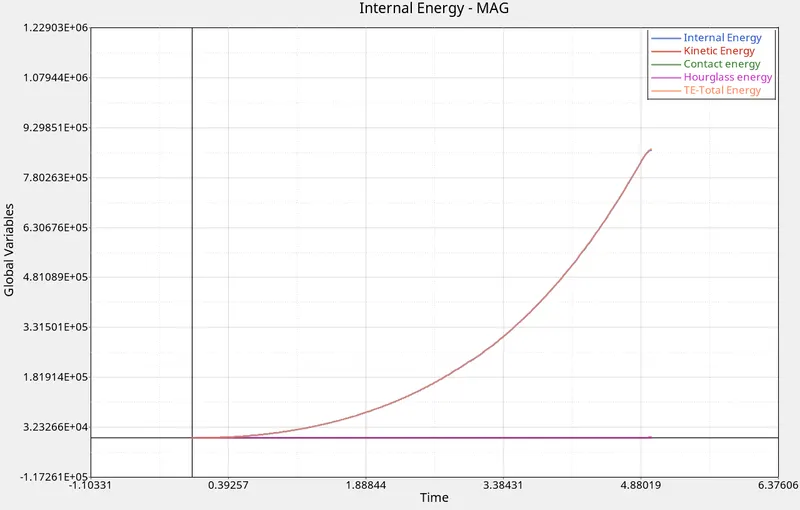
• This Energy graph is in a controlled way as this is the .rad file of no failure card model .
• From this energy graph we can observe that Only Total energy & Internal energies graph is slowly & progressively increasing and all other energies like KE , Contact & Hourglass energy are near the X axis line .
• Next we will be plotting graphs for Rwall forces as -
• Start the new plot by going to File - New - Plot - The new hypergraphs page will be created
• Than here in X type select as Time and Y type as Rigid wall - 1 Punch - Than select Fx , Fy , Fz , Total forces , Total resultant forces etc.. should be plotted on the graph.

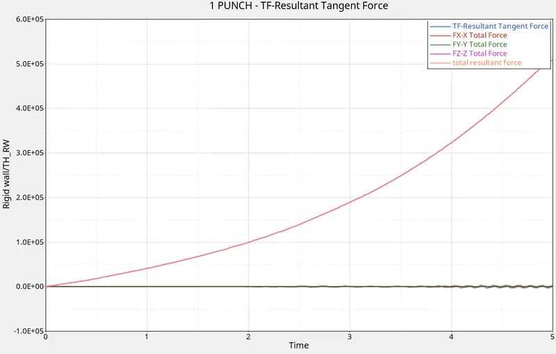
• By this RW graph we can observe that Total Force in Fzz & total resultant force are increasing gradually and properly and goes very high upto some extent and stops but other all forces will be lying near the X axis line with very clean representation with very even lines.

Conclusion:

By performing whole procedure in step by step manner we will get to know the energy values , rigid wall force values indicated graphically and also Energy error & mass error , Total no. of cycles , Time step , Total elapsed time .....these all values can be known and .Rad file of this case will be used for next case to know consequences after certain changes.

CASE 6

Objective:

The main objective in Case 6 is to run the model by changing material model to Law 36(M36_Plas_Tab) & save it with the name Law36 Plas_Tab with change of values as mentioned in the quesion video file as same E , n , Nu Rho etc.. values & than creating Energy graphs & Rigid wall curves and observe how the transformation is going on.

Given,

E = 71000

Eps_P_max = 0.16

Epa_t1 = 0.1

Epa_t2 =0.11

Density = 0.0027

Nfunc = 1

Fsmooth = 0

Fpscale = 1

Fcut = 0

Procedure:

• Here .Rad file will be taken from previous case out file as -
• Go to File - Import - Solverdeck - Select the previous Case 5 file from the location where it is saved- from that select .001 rad file -Click on Import
• After Importing go to model tab and check all the values than
• Rename the card to Law36 Plas_Tab
• Here we will be changing Card image from M2_Plas_Johns_Zeril to M36_Plas_Tab .
• After this update with all values of E , Rho , Nu values as before in this M36_Plas_Tab card image dropdown with given values in question.

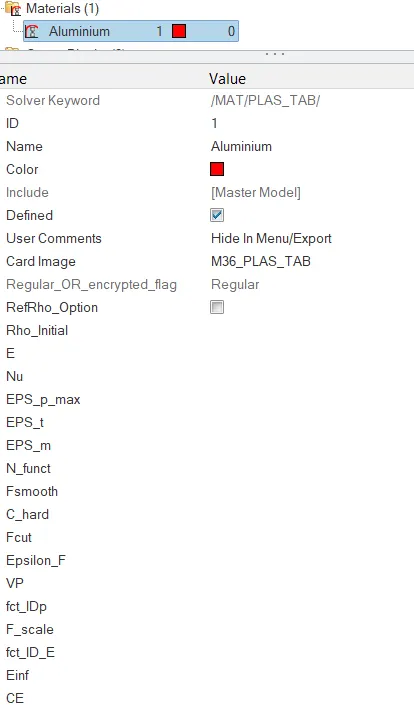
• Than near fct_IDp it asks to select a curve now -
• Go to Curve card - Create a new curve card - Rename it accordingly - Than by using the X and Y values in the question file create a curve graph than attach this in the Function Id .
• After creating a curve card it will look like this -

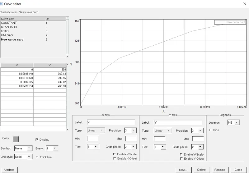
• Now Go to Analysis - Radioss - Select the location where the files should be saved
• Keep Export options:all , Run options: analysis , run number: 1 , Options : -nt 4
• Than hit on Radioss option it starts simulation of the file
• Now we will be getting a Out file as shown below open this in notepad

• After a certain time the simulation running will stop than go through those and there Total no. of cycles , Energy error & Mass error , Total starter run time , engine run time all these values can be taken from there.
• After observing all these values note those values properly.

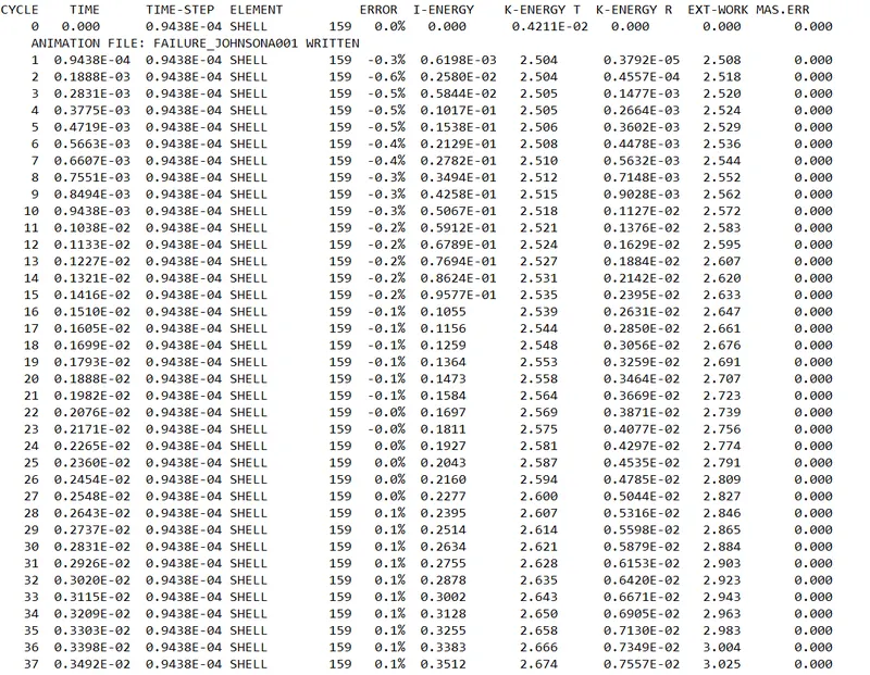
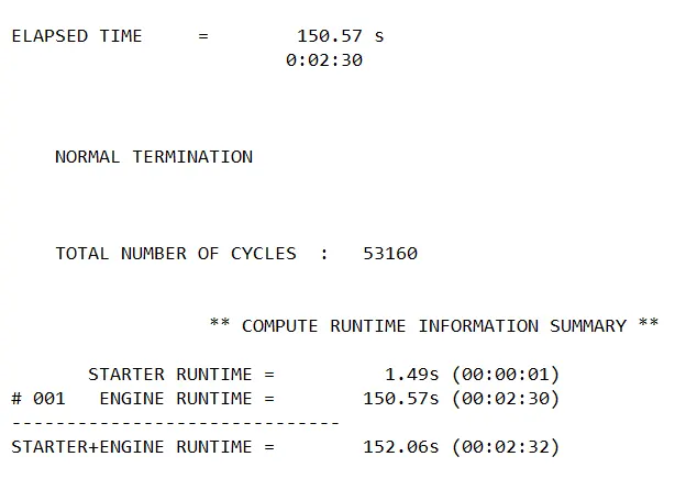
From above we can know,

Total no. of cycles = 53160

Elapsed time = 150.57 sec

Max. Positive energy error = +0.6%

Min . Negative ernergy error = -0.1%

Mass error. = 0.000

• From this we can get to know that the positive energy is less than 2% which is accceptable incase of QEPH & Fully integrated element properties and also Min energy error is always acceptable as it means the amount of energy which is dissipated.
• Here coming to Mass error it is 0 as here no mass is added to meet specified time step.
• Than select a Multi page option and in new page selct Hyperview.
• Select the .h3d files for case 5 worked and import that in Hyperview window
• After importing there will be a Ball and circular plate type model present on the screen
• Start working on the model
• Switch on the mesh using shaded elements & meshlines option
• Than by using contour option vonmises stress is applied & indicated on the model and by using animation option we can test how the crash is happening & how is it failing can be anlysed.

BEFORE FAILING

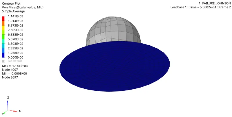
AFTER FAILING SHOWN THROUGH VONMISES STRESS

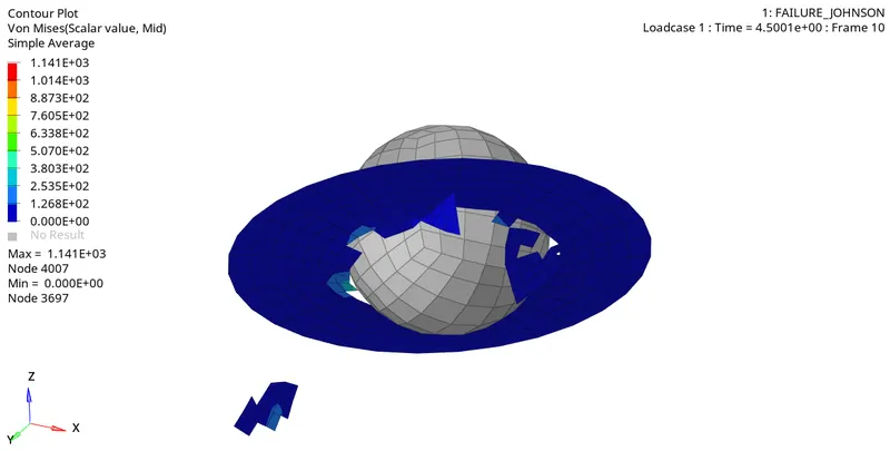
• As here we have used the .rad file of previous file isused and with Material model M36_Plas_Tab is used as this means it is a plastic model there is very high chance of elements deleting here the elements will be deleted due to the brittleness.
• Next by using hypergraphs 2D plot the Energy graphs and Rigid wall forces as
• Go to hypergraphs - Select the T01 file to plot the graphs than-
• Select X type - Time & Y type - Global variable - Select the type of energies to be plotted on the graph -than select MAG - Click on Apply.
• Here we will select Internal energy, Kinetic energy , Contact energy , total energy, hourglass energy etc...than the graph will be plotted.

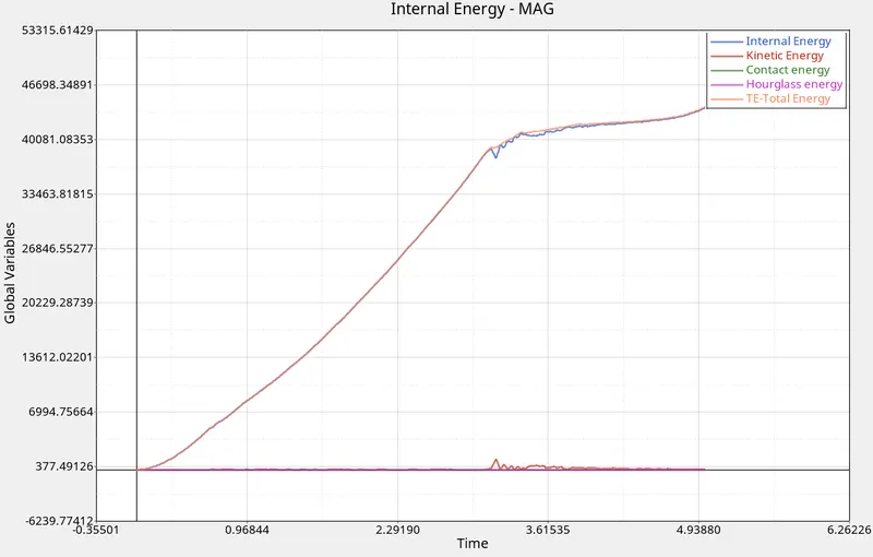
• This Energy graph is in a controlled way as this is the .rad file of no failure card model .
• From this energy graph we can observe that Only Total energy & Internal energies graph is slowly & progressively increasing and in middle there is a slight disturbance like small waves and all other energies like KE , Contact & Hourglass energy are near the X axis line .
• Next we will be plotting graphs for Rwall forces as -
• Start the new plot by going to File - New - Plot - The new hypergraphs page will be created
• Than here in X type select as Time and Y type as Rigid wall - 1 Punch - Than select Fx , Fy , Fz , Total forces , Total resultant forces etc.. should be plotted on the graph.

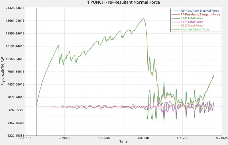
• By this RW graph we can observe that Total Force in Fzz & total resultant force are increasing gradually andwith lot of disturbances and goes very high upto some extent and stops but comes down towards X axis in last stage, other all forces will be lying near the X axis line representation with disturbed wavy lines.

Conclusion:

By performing whole procedure in step by step manner we will get to know the energy values , rigid wall force values indicated graphically and also Energy error & mass error , Total no. of cycles , Time step , Total elapsed time .....these all values can be known and .Rad file of this case will be used for next case to know consequences after certain changes.

CASE 7

Objective:

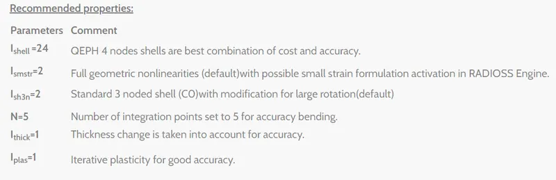
The main objective in Case 7 is to downlown the Law27 .rad file from the question file & run the model as Law 27(M36_Plas_Tab) & save it with the name Law36 Plas_Brit with change of values as mentioned in the quesion video file as it should have reccomended element property values which are done in previous challenge same E , n , Nu Rho etc..as values & than creating Energy graphs & Rigid wall curves and observe how the transformation is going on.

Procedure:

• Here .Rad file will be taken from previous case out file as -
• Go to File - Import - Solverdeck - Select the previous Case 5 file from the location where it is saved- from that select .001 rad file -Click on Import
• After Importing go to model tab and check all the values than
• Rename the card to Law27 Plas_Tab
• Here automatically we will be getting changed Card image from beginning only as the new .rad file is imported.
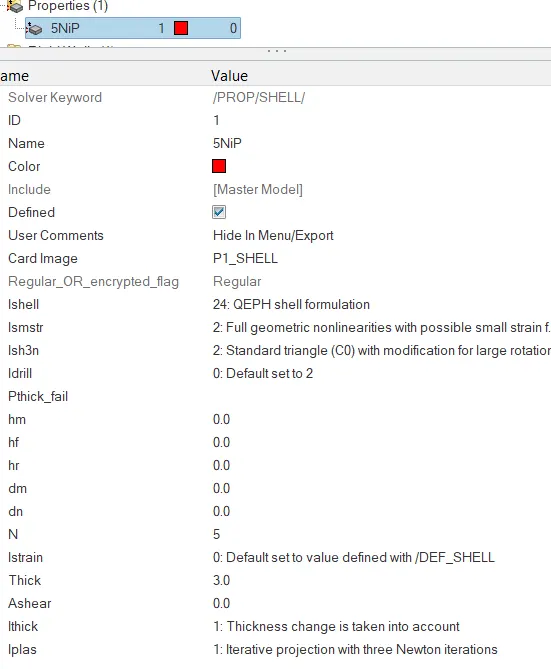
• After this update with all values of E , Rho , Nu values as with reccomended element properties in this M27_Plas_Brit card image dropdown with given values in question.
• Change the Ishell , Ismstrn ,...with reccomende values ne Properties card as -

• Now Go to Analysis - Radioss - Select the location where the files should be saved
• Keep Export options:all , Run options: analysis , run number: 1 , Options : -nt 4
• Than hit on Radioss option it starts simulation of the file
• Now we will be getting a Out file as shown below open this in notepad

• After a certain time the simulation running will stop than go through those and there Total no. of cycles , Energy error & Mass error , Total starter run time , engine run time all these values can be taken from there.
• After observing all these values note those values properly.

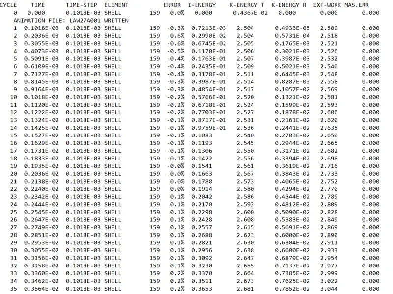
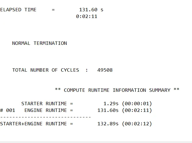
From above we can know,

Total no. of cycles = 49508

Elapsed time = 131.60sec

Max. Positive energy error = +1.1%

Min . Negative ernergy error = -0.0%

Mass error. = 0.000

• From this we can get to know that the positive energy is less than 2% which is accceptable incase of QEPH & Fully integrated element properties and also Min energy error is always acceptable as it means the amount of energy which is dissipated.
• Here coming to Mass error it is 0 as here no mass is added to meet specified time step.
• Than select a Multi page option and in new page selct Hyperview.
• Select the .h3d files for case 5 worked and import that in Hyperview window
• After importing there will be a Ball and circular plate type model present on the screen
• Start working on the model
• Switch on the mesh using shaded elements & meshlines option
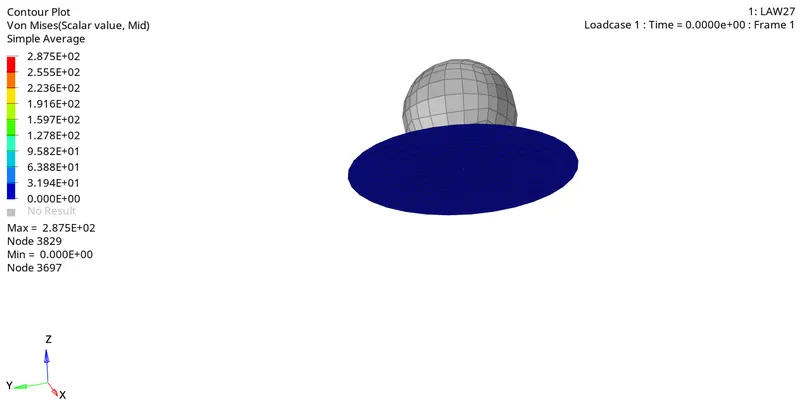
• Than by using contour option vonmises stress is applied & indicated on the model and by using animation option we can test how the crash is happening & how is it failing can be anlysed.

BEFORE FAILING

AFTER FAILING SHOWN THROUGH VONMISES STRESS

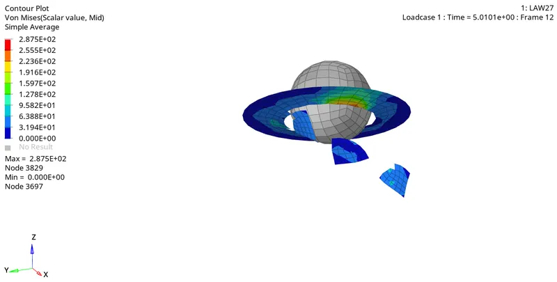
• As here we have used the .rad file of previous file isused and with Material model M27_Plas_Brit is used as this means it is a plastic model there is very high chance of elements deleting here the elements will be deleted due to the high brittleness.
• Next by using hypergraphs 2D plot the Energy graphs and Rigid wall forces as
• Go to hypergraphs - Select the T01 file to plot the graphs than-
• Select X type - Time & Y type - Global variable - Select the type of energies to be plotted on the graph -than select MAG - Click on Apply.
• Here we will select Internal energy, Kinetic energy , Contact energy , total energy, hourglass energy etc...than the graph will be plotted.

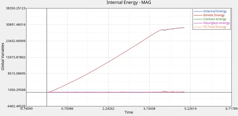
• This Energy graph is in a controlled way as this is the .rad file of no failure card model .
• From this energy graph we can observe that Only Total energy & Internal energies graph is slowly & progressively increasing and in middle there is a slight disturbance like small waves and all other energies like KE , Contact & Hourglass energy are near the X axis line .
• Next we will be plotting graphs for Rwall forces as -
• Start the new plot by going to File - New - Plot - The new hypergraphs page will be created
• Than here in X type select as Time and Y type as Rigid wall - 1 Punch - Than select Fx , Fy , Fz , Total forces , Total resultant forces etc.. should be plotted on the graph.

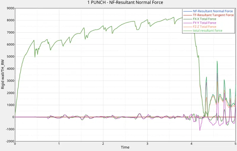
• By this RW graph we can observe that Total Force in Fzz & total resultant force are increasing gradually andwith lot of disturbances and goes very high upto some extent and stops but comes down towards X axis in last stage, other all forces will be lying near the X axis line representation with disturbed wavy lines.

Conclusion:

By performing whole procedure in step by step manner we will get to know the energy values , rigid wall force values indicated graphically and also Energy error & mass error , Total no. of cycles , Time step , Total elapsed time .....these all values can be known and .Rad file of this case will be used for next case to know consequences after certain changes.