Assignment 4-RADIOSS Material Laws Challenge

OBJECTIVE :

To apply different material formulations, property changes in the simulation model and compare the behaviour of the elements, compare the total no.of cycles, energy and mass error, total simulation time etc with the changes made in the material law and properties.

PROCEDURE :

Case 1 : Default Parameters ( Law 2 with Eps_max Failure)

Go to the Hypermesh window, Open the Failure_0000.rad file in the Hypermesh window and keep the properties of the elements to the best required settings.
These are the changes which are made to the shell element properties.


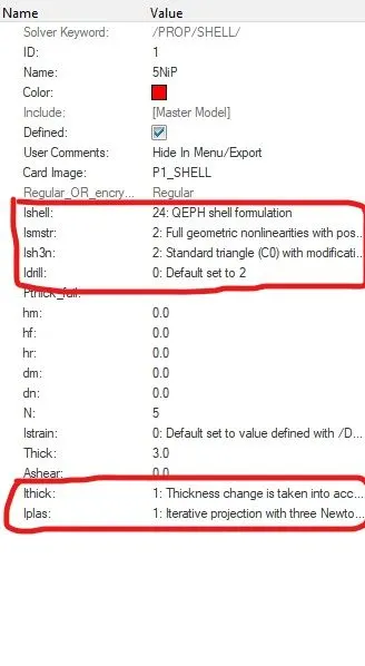
We can see that the material assigned and the failure card assigned to the elements as default:



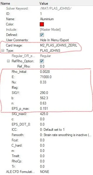
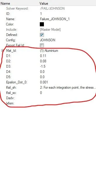
With all these parameters set, we can start the analysis. Go to Analysis >> Radioss >> Save the file as ( as per required ) >> Enable connectors >> Options >> -nt 4. Then click on Radioss to run the simulation. We can then view the total elapsed time, no.of cycles, energy error etc




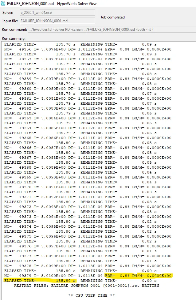
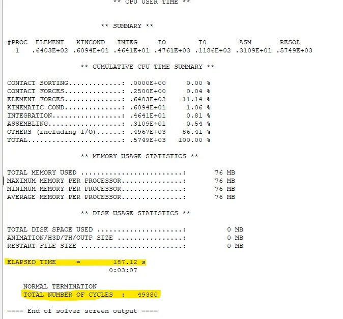
Here we can see that the Energy error is 0.8% and the mass error is 0. This means it is well within the acceptable range of 5%
Also the total time is about 187.12s and the total cycles were 49380.


Now, open the .h3d file in the Hyperview and the T01 file in the Hypergraph to see the contours and the plots of the global variables.
On seeing the Vonmises contour plot, we can observe :





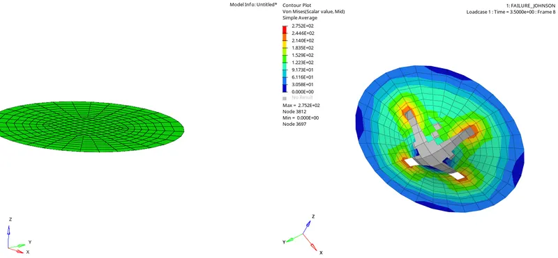
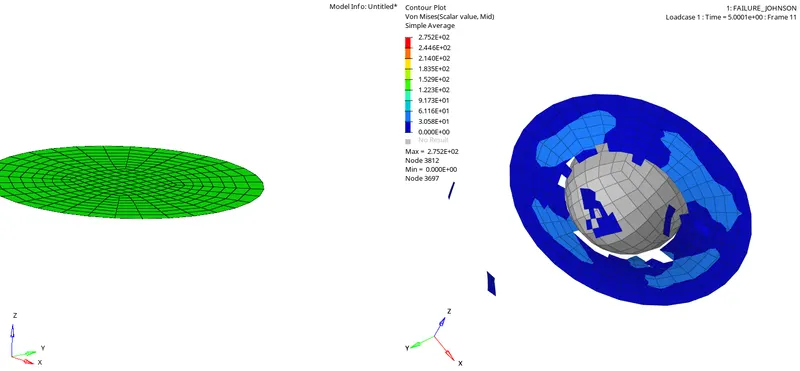
The material law 2 - Johnson cook failure model is used here in which the stresses were calculated as the function of strain,strain rate and the temperature change.
We can see that the maximum stress produced is about 275Mpa and the elements were deleted since we have given the Eps max failure as 0.151.
This means the elements in which If the integration points reaching 15.1% of the plastic strain would be deleted. Also there were Eps value for tensile and compressive strain seperately. If the elements reaches any of those value or they collectively reach 15.1% of plastic strain then the elements would be deleted.
The Yield stress provided was about 290Mpa and the maximum stress produced was 275Mpa.We can see that the elements were being deleted after it reaches 15.1% of the plastic strain.
Since the Ixfem was 0 in this model, once the elements reaches the failure strain it is getting deleted.

Now, we load the T01 file in the Hypergraph to see the behaviour of the global variables:



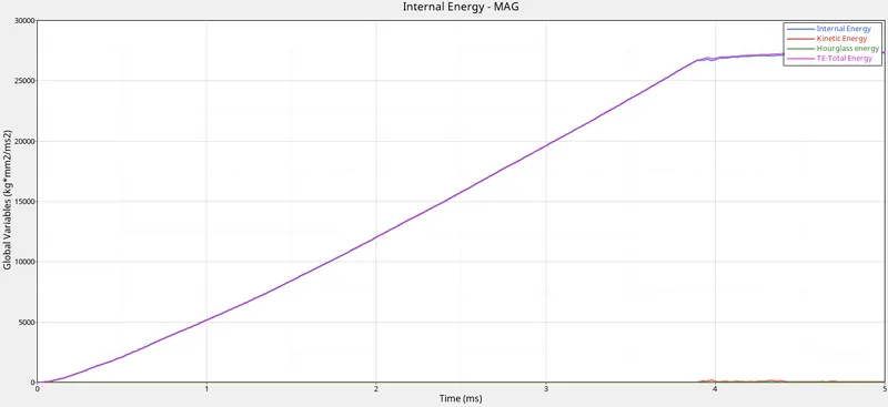
We can see a slight spikes around 4ms in both the internal energy and the total energy. There is no hourglass energy due to the usage of QEPH elements. The internal energy and the total energy were increasing by time as the elements were absorbing the energy as they deform.

Case 2 : Law2 Eps_Max_Crack

In this case we are going to change the /Failure_Johnson_1 card parameters. These are the required changes to be done on the failure card :


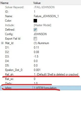
Since we have set the Ixfem :1, the elements would be cracked and the Ifail_sh : 1 sets the failure shell element to be cracked or deleted.
The Dadv would enhance the crack formulation of the elements. Now this condition should be solved in the solver and then we can see the changes in the simulation and its result.



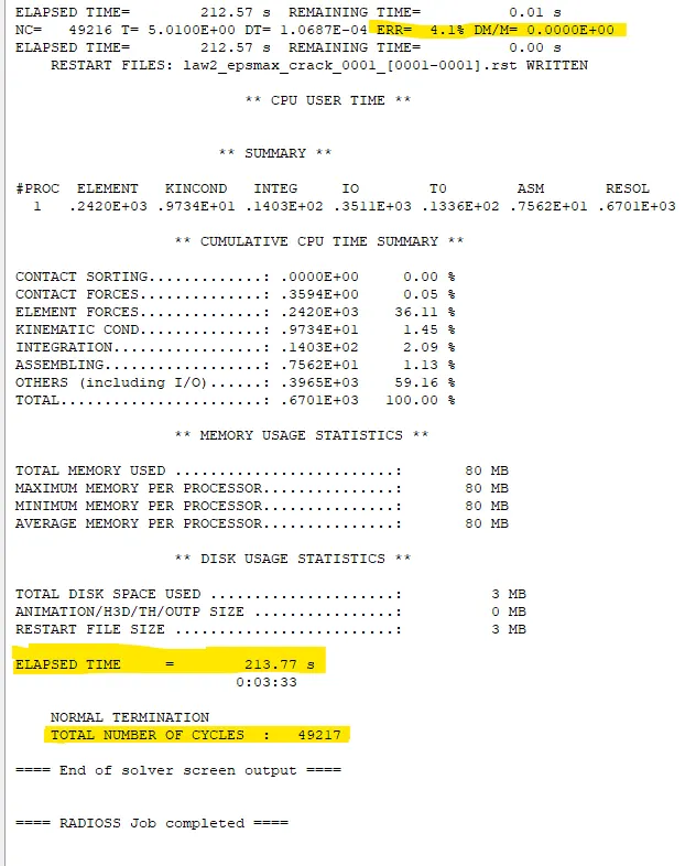
Here we can see that the energy error is 4.1% and the mass error is 0 which is very well within the acceptable range. The total time elapsed was 213.77s and the no.of.cycles is 49217.
This shows that the total time consumption and the energy error is higher than that in the previous case.

Now, Open the.h3d file in the Hyperview to see the simulation and the stresses produced in the elements.







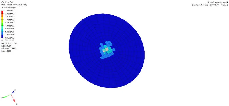
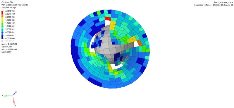
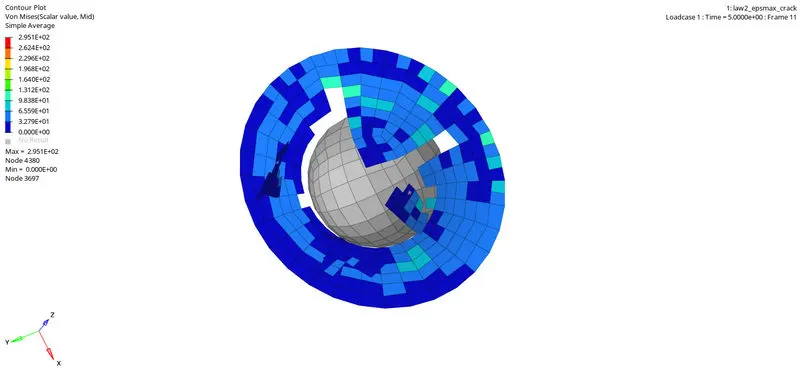
We can observe that the elements were getting cracked in the initial stage which is not the case in the previous simulation. This is due to the fact we have enabled the Ixfem option and the Ifail_sh is set to 1 which in turn enables the shell elements to crack before deleting.
The maximum stress in the simulation is found to be 295.1Mpa which is greater than the previous case.

Now, open the T01 file in the Hypergraph to check the global variables like internal energy and total energy in the simulation.



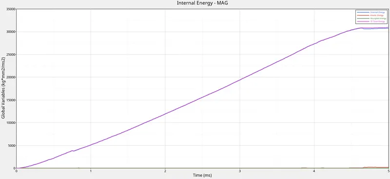
Here we can see that the Total energy and the internal energy gradually increasing over the time. The internal energy is above 30000kg.mm^2/ms^2 which is higher than the previous case since we have elements which are cracking initially and then getting deleted which provides a path to absorb more energy.

Case 3 : Law2 Eps_max_nofail

In this case, all the failure conditions which were entered previously have been deleted by deleting the /Failure_Johnson card in the cards section.
Now, solve this case in the solver and see what are the changes in the simulation and the results.



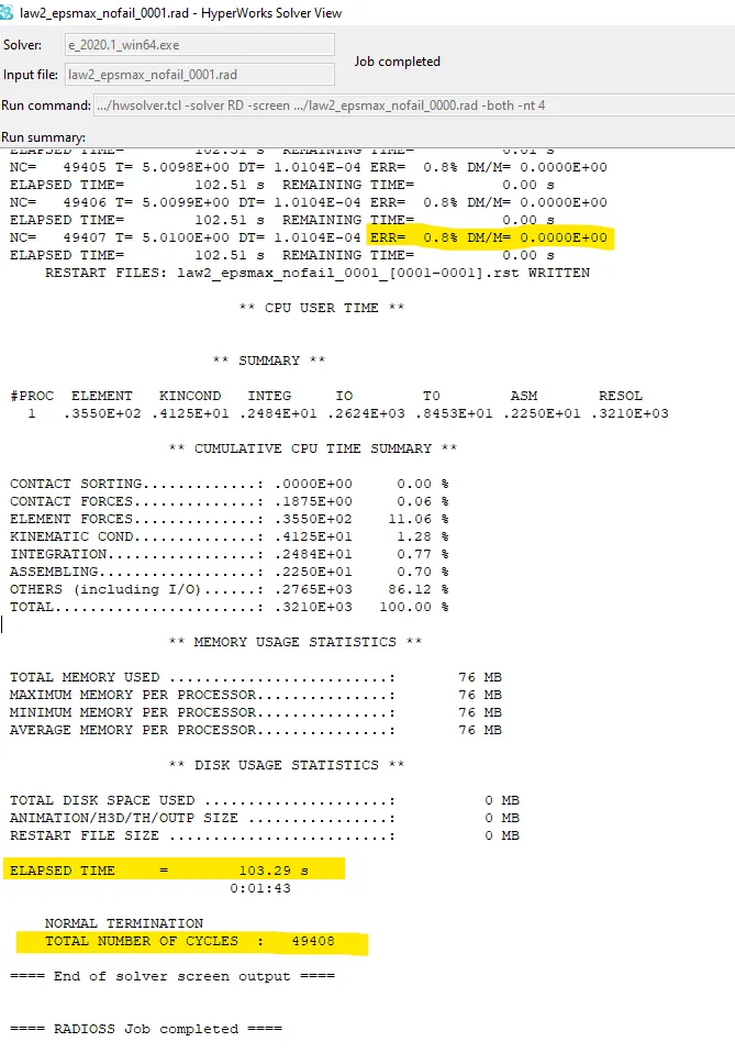
Here we can see that the energy error is 0.8% and the mass error is 0. These values are under the accpetable range. The total time taken was about 103.29s which is less than the other two case and the total number of cycles is 49408.


Now, open the .h3d file in the Hyperview and open the vonmises contour to see the stress produced in the simulation.



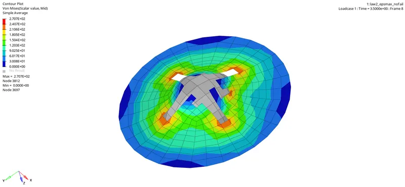
Here we can see there are no cracks in the elements, The total stress in the simulation is about 270Mpa. Since the failure card is deleted, It follows the Law 2 in which the Eps max value is provided. This means the elements integration point upon reaching the value of the Eps max would fail and gets deleted.

Now, Open the T01 file in the Hypergraph to check the internal energy, hourglass and the total energy produced in the simulation.



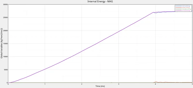
The Internal energy and the total energy were increasing gradually as the time goes on which is quite similar to the other cases. The Hour glass energy is zero since the QEPH type shell formulation is provided.

Case 4 : Law2_no_Eps_max

In this case, we are changing the Eps_max value from 0.151 to 0. This means the Elements would not be deleted even if any one of the integration point reaches the respective value, This inturn implies that the elements were free from deletion and since we kept the Eps max value to 0, It would take the default value of 10^30 which inturn is almost never reachable in this case. The elements would reach the plastic strain and would never fail.



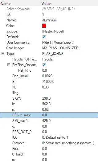
Now, run the simulation in the radioss solver and check the energy and mass error and check if they are under the acceptable range.



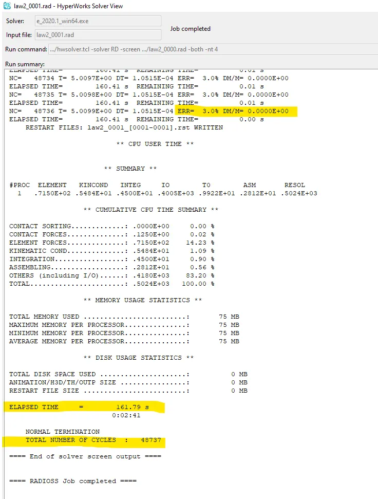
After running, we can see that the energy error is about 3.0% and the mass error remains 0. The total time taken is 161.79s and the total no.of.cycle is 48737.
These values were within the acceptable range.

Then, open the .h3d file in the Hyperview as we do and check the simulation and the stress produced in it.



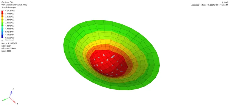
Since we have kept the Eps max failure value to default, we don't see any elements failing and getting deleted. The maximum stress in the simulation is about 424.7Mpa which is much higher than the other cases. Since we have set the SIG max value to 425Mpa, the stress build up was about closer to that value. No elements were deleted in this simulation.

Lets's see the energy plots by loading the T01 file in the Hypergraph.



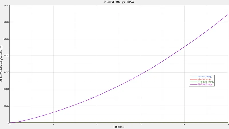
In this case, the energy were increasing exponentially and there is no hourglass energy. Since there is no deletion of elements, the Internal energy increases and the total energy is found much higher than 60000Kg.mm^2/mm^2
The kinetic energy is flat since there are no elements which were failing for the plastic strain value.


Case 5 : Law 1

In this case, the complete material law is changed from Law 2 Johnson cook to Law 1 Isotropic Elastic material. This should be done in the materials card section and the value of initial density, young's modulus and the poisson's ratio has been carried over from the previous cases.



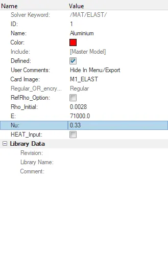
Once these changes has been made we can run the model in the radioss solver and check the changes in the energy error and the mass errors.



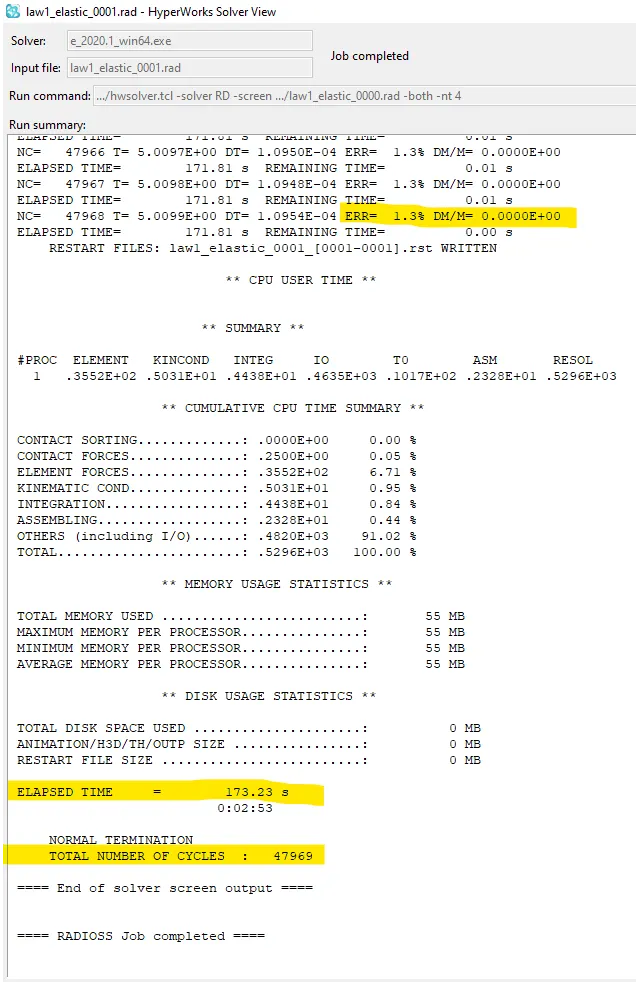
We can see that the energy error is about 1.3% and the mass error is 0. The total time taken in the simulation is 173.23s and the total no.of.cycles is 47969
With all the values considerable we can now open the .h3d file in the Hyperview to look at the simulation and the stress produced.



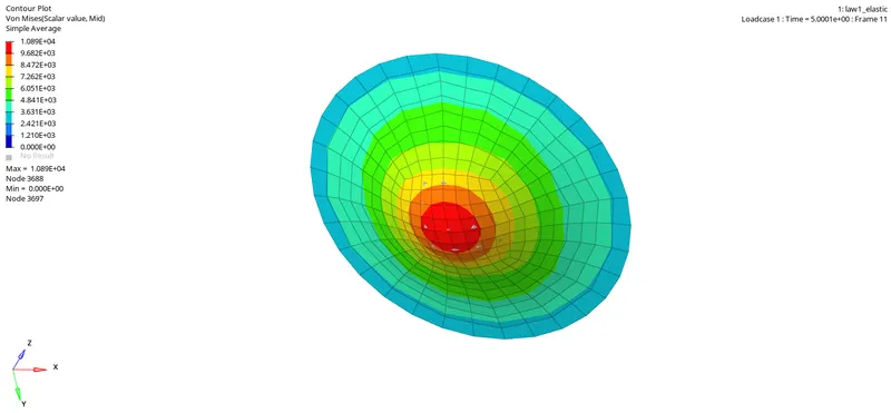
In this case, since the material is defined as the elastic material, the elements would not enter the plastic strain stage. Thus there is no maximum plastic stress produced and there are no elements which were failing and deleted. Though we can see some elements penetration in the simulation, that is due to the fact that the contact points were not defined in the model.

Now, let's see the energy plots in the Hypergraph by loading the T01 file in the Hypergraph window.



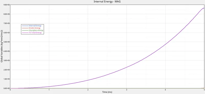
Here, the internal energy and the total energy were increasing exponentially with the time. There is no hour glass energy in this simulation.


Case 6 : Law 27

Now, open the law27_0000.rad file in the hypermesh window and set the properties and the material parameters.
In this Law 27 which is called as the Elasto plastic Johnson cook model with orthographic brittle failure material which combines the Johnson cook material with the brittle failure material. There are certain alloys are composites which are though elasto plastic, they would have the brittle failure characteristics. Such properties would be defined in this law.

The elements & material properties were formulated as usual as follows :



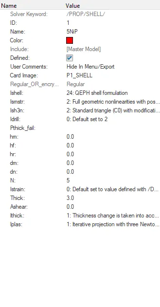
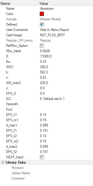
The Law has been changed to Law 27 Plas_Brit in which the density, young's modulus, poisson's ratio were carried over and the SIG Y value is seem to be 290Mpa. The other values are of :

EPS_t1 : Tensile failure strain at which stress starts to reduce in principal strain direction 1
EPS_m1: Maximum tensile failure strain in principal strain direction 1 at which the stress in the element is set to a value dependant of dmax1
EPS_f1 : Maximum tensile strain for deletion of element in principal strain direction 1
d_max1: Maximum damage factor in the principal strain direction 1 which is at default value of 0.999
Similarly, the EPS_t2, EPS_m2, EPS_f2 and d_max2 corresponds to the direction 2.

With all these values changed, run the simulation in the radioss solver and then check the results.


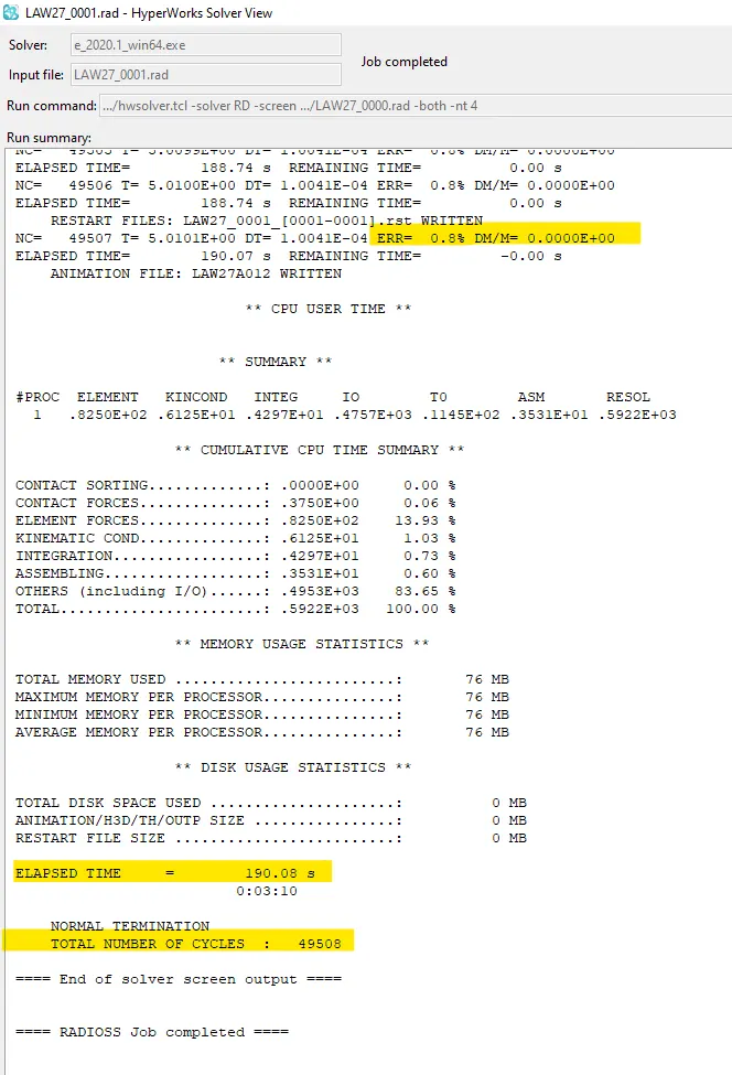
We can see that the energy error is about 0.8% and the mass error is 0. The total time consumption is 190.8s and the total no.of.cycles is 49508.
These values are considerable and are within the acceptance range.

Now, load the .h3d file in the Hyperview to see the simulation and the stress produced in it.



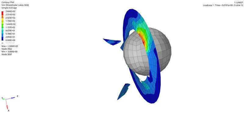
The maximum stress in the simulation is about 260.4Mpa which is lesser than the provided SIG Y value 290Mpa, the elements were deleted after the intergration points reach the failure value in the principal strain direction according to the values provided in the EPS_t1,t2 etc.,
Here the material would fail only for the tension and the elements were being deleted like the brittle failure.

Now, let's see the energy plots by opening the T01 file in the Hypergraph.



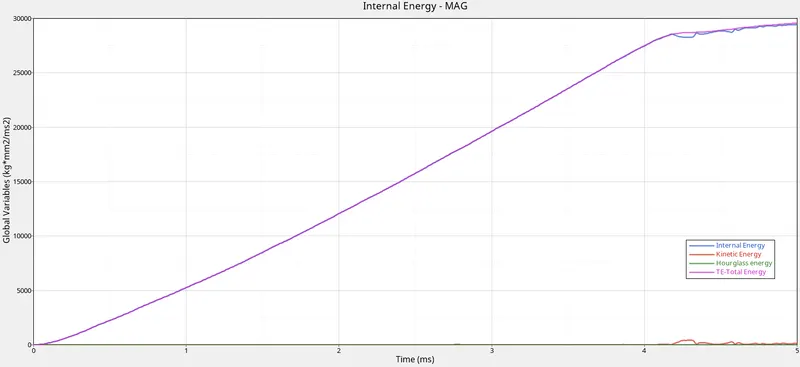
The internal energy increases exponentially and after 4ms, there are slight ups and downs which indicates the elements being deleted like the brittle failure.


Case 7 : Law 36

In this case, again open the Failure_Johnson_0000.rad file and change the Material paramaters from Law 2 to Law 36 which is Elastic Plastic Piecewise Linear material which provides the option to manually load the work hardening portion of the stress-strain behaviour of the material.

Firstly, go to the curves card section >> right click and create >> Curve >> Enter the x and y coordinates corresponding to the Stress and strain value as in the usual stress-strain graph. Then save the curve.

Now, go to materials card, enter the N_function as 1 and change the Function ID by selecting the curve ID which is created before. Thus we can set the stress strain curve for the material with our own values.



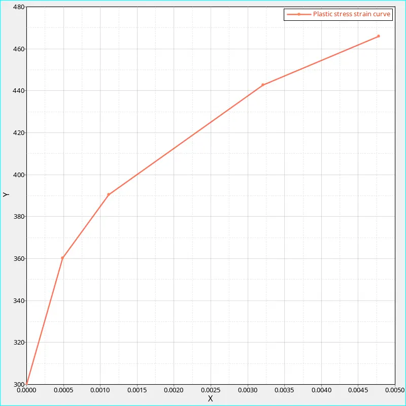
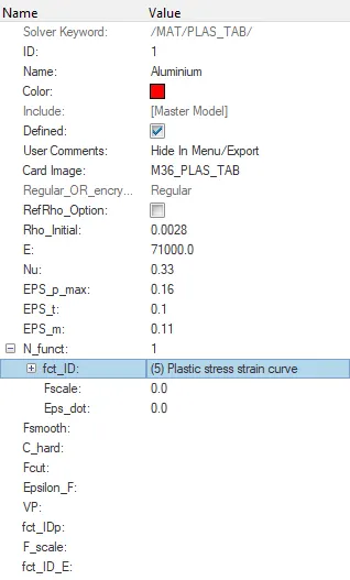
With all these parameters set, we can now run the simulation in the radioss solver to check the results and the simulation.



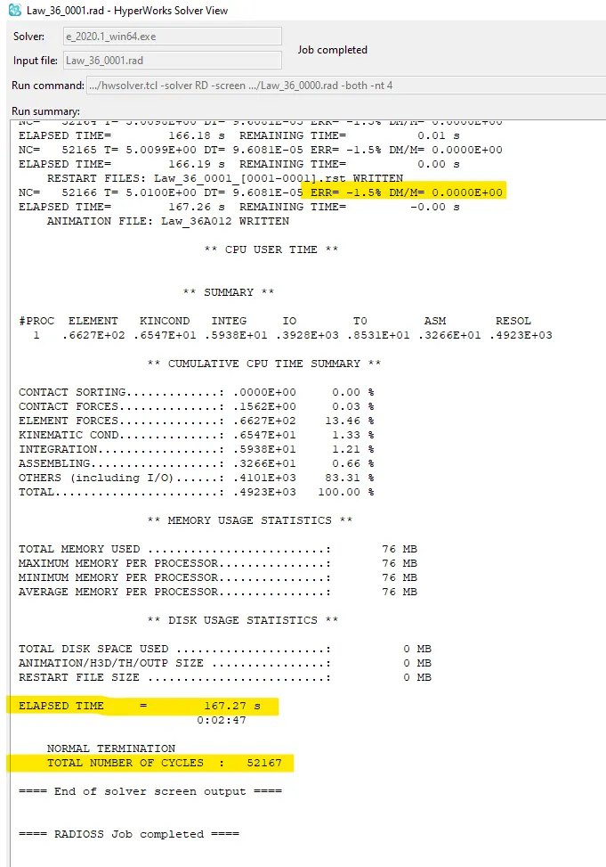
We can see that the energy error is -1.5% and the mass error is 0 which is desirable. The total time taken is 167.27s and the total no.of.cycles is 52167
Now, let's see the simulation and the contour of the stresses produced by opening the .h3d file in the Hyperview.



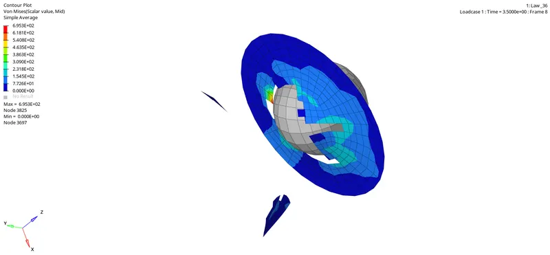
We can see that the maximum stress produced in this case is about 695.3Mpa which is higher than all the other cases and we can see that the elements were being deleted as they reach the maximum stress value and some deleted at the Eps_f value which is the failure value according to the true stress-strain curve which is obtained from lab experiments and are fed in to the solver using the Law 36.

The law36 which is piecewise linear elastic plastic material gives us the flexibility of setting the work hardening portion of the material in the stress-strain curve for different strain rates. It depicts the behavior of the stress and strain after the Yield point in which yield point is set to 0.
The failure of the elements and its deletion follows the following graph:

Now, load the T01 file in the Hypergraph to view the Energy plots by following the similar opening methods.



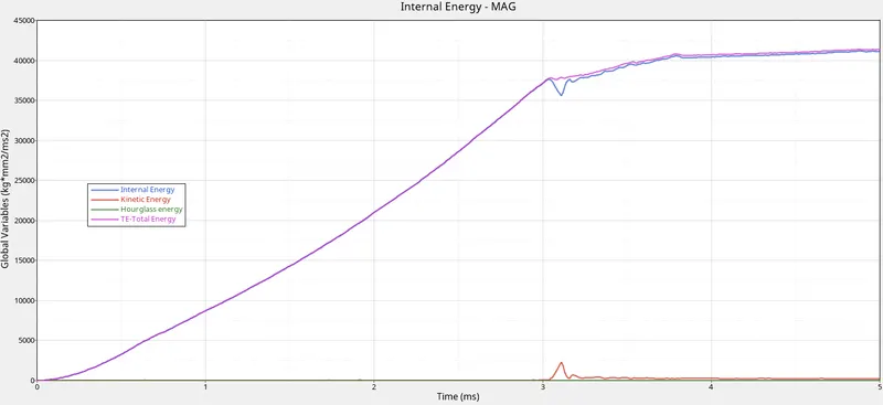
We can see that there are slight ups and downs after 3ms, which depicts the fact that the elements were being deleted as they were reach the failure criteria. The total energy and the internal energy were increasing exponentially and they are found to be above 40000Kg.mm^2/ms^2

Thus, we have run the simulation with various material parameters and its changes in the results has been observed.

RESULTS :

Case	Total no.of.cycles	Total time taken (s)	Energy error (%)	Mass error	Maximum stress value (Von-mises) (Mpa)
Law 2 Eps_max_failure	49380	187.12	0.8	0	275
Law 2 Eps_max_crack	49217	213.77	4.1	0	295.1
Law 2 Eps_max_nofail	49408	103.29	0.8	0	270
Law 2 no_Eps_max	48737	161.79	3.0	0	424.7
Law 1 Elastic	47969	173.23	1.3	0	1089
Law 27	49508	190.08	0.8	0	260.4
Law 36 _plas_tab	52167	167.27	-1.5	0	695.3

Based on all the simulations and the results produced, the Law 27 (case 6) gives realistic simulation for the brittle material failure while the Law 36 would provide more accurate results as they have the manual intervention over stress strain curve behaviour determination. The other failure modes has their own significance. The Case 6 is found to be quite natural with its simulation as they have the crack propagation in the direction of mesh for the given simulation scenario.

Thus, we have learnt :
1. About commonly used Material laws.
2. How to apply material laws and how to view the results and simulation.
3. Comparison of the material law and their significance.
4. Various constants being calculated in different material laws.
5. Plotting the Stress,displacements & global varaibles in Hyperview and Hypergraph.