Material Laws in RADIOSS

AIM

This work aims to inspect the variations coming up in the results of the simulation, with the changes in material properties.

OBJECTIVE

1. To run the model with appropriate element properties, and with law 1
2. To run the model as it is.
3. In /FAIL/JOHNSON, to change Ifail_sh=1, Dadv=1, and Ixfem=1, and run the model as Law2_epsmax_crack.
4. To delete /FAIL/JOHNSON card/, and run the file as Law2_epsmax_nofail.
5. To delete the value of EPS_p_max and run the model with the name Law2.
6. To convert the existing material model to Law1 elastic with the same density, E, nu, and run the model.
7. To open LAW27_0000.rad, change its shell properties to recommended shell properties, and run the model with the name Law27.

CASE 1: LAW 1

In the first case, the model was simulated with a law 1 material card image. Using the law 1 card image, the behavior of material deformation remains in the linear elastic region. It follows Hooke’s law i.e., a linear relationship between stress and strain. And therefore, when the result of the simulation is analyzed, it shows no failure in the model, irrespective of the value of stress, which is beyond the material yield stress value. Fig. 1 shows the contour plot of VonMises Stress with the simple averaging method. The maximum value of VonMises stress generated in this case is 1.089E+04.

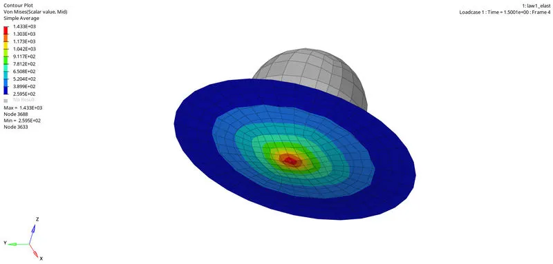
Figure 1: Simulation of the model with LAW 1 (/MAT/ELAST/) material card image.

It is recommended that the law 1 card image should be used when it is certain that the material deformation wouldn’t deform beyond the material yield stress value, as in the case of small-displacement vibration, or small loading cases.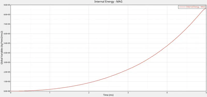

Figure 2: Internal energy vs. time plot for case 1.

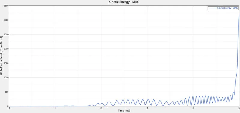
Figure 3: Kinetic energy vs. time plot for case 1.

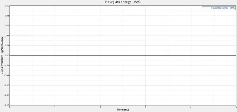
Figure 4: Hourglass, and contact energy vs. time plot for case 1.

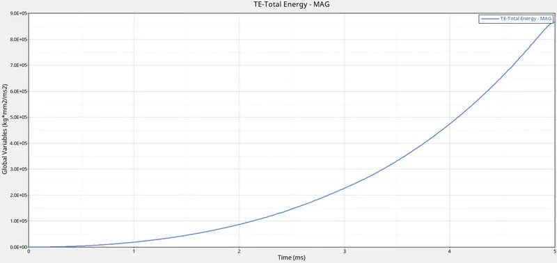
Figure 5: Total energy vs. time plot for case 1.

Fig. 2 shows the plot of internal energy vs. time graph. The internal energy is the function of displacement, therefore, with the continuous expansion of an aluminum plate, there is a continuous change in the internal energy.

The value of kinetic energy is very negligible compared to internal energy. However, it shows that as soon as the aluminum ball came in contact with the aluminum plate, the change in kinetic energy can be seen. The ups and downs in the kinetic energy might be because of the elastic nature of the aluminum plate. This fluctuation is damped around 4.6 s of simulation time. This might be because of the stretch in the aluminum plate, which further constrains the movement of the element.

The hourglass energy is zero because of the improved shell elemental properties. The total energy shows the replica of internal energy.

CASE 2: Law2_epsmax_failure

Law 2 is for the PLAS_JOHNS material card which represents the Johnson-Cook model. The Johnson_Cook model takes the value of stress as a function of strain, strain rate, and temperature. Using this material card, the model behaves as an elastic-plastic model. Figure 6 shows the simulation of the model with eps_max failure.

In this case, the value of EPS_p_max or is defined and given the value equal to 0.151. The EPS_p_max is the value of the maximum strain to which the material can deform. The 0.151 value of strain, or 15.1% value of strain when crossed, the elements that crossing the limit gets deleted, to interpret the real-time scenario. However, the mode of failure is not so similar to the real-time scenario, as can be seen in fig. 6. The max. value of VonMises stress generated in case 2 is 275.2 MPa.

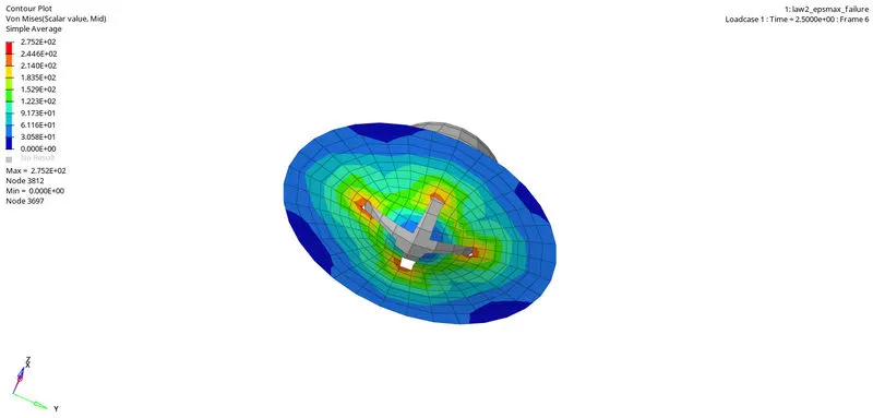
Figure 6: Simulation of the model with law 2 material card image, defining the value for EPS_p_max = 0.151.

The law 2 card image is recommended when there are chances of material deformation crossing the yield point. Also, the failure can be seen for shell elements only, and not 3d elements.

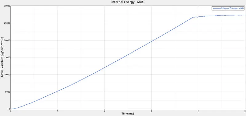
Figure 7: Internal energy vs. time plot for case 2.

The internal energy kept increasing till 3.8 or 3.9 ms, as the aluminum sheet continue to stretch but as soon as the elements crossed the EPS_p_max value of 0.151, after 4 ms of time, there is no change in internal energy can be seen because the failed elements started deleting, and not many elements remained in contact with the ball.

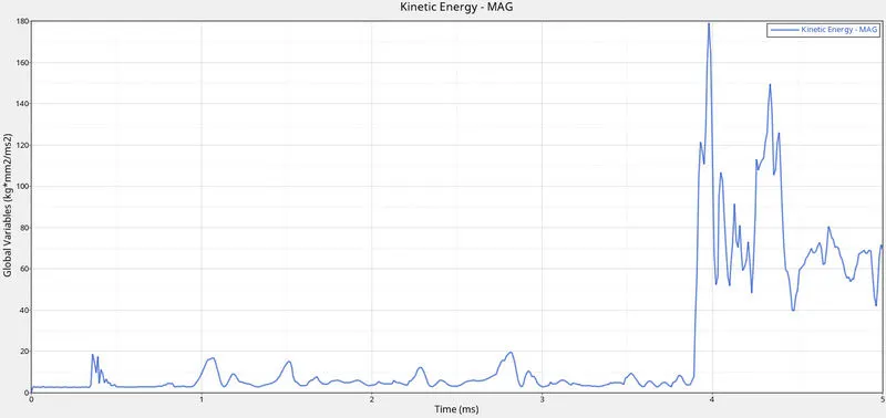
Figure 8: Kinetic energy vs. time plot for case 2.

The kinetic energy is negligible until the elements started failing. Once the elements started failing, some of them disconnected and threw out of mesh with some velocity. This increases the kinetic energy which can be seen in fig. 8, after 3.8 or 3.9 ms.

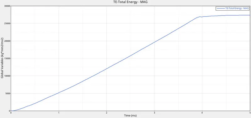
Figure 9: Total energy vs. time plot for case 2.

The value of kinetic energy is very small as compared to the internal energy, and therefore the total energy is the replica of the internal energy itself.

Figure 10: Hourglass energy vs. time plot for case 2.

The hourglass energy is zero because of the improved shell elemental properties.

Case 3: Introduction to Ixfem

The elements when failed using Johnson-Cook material card image, they got completely deleted, which is not represented as a real-time scenario. So, to bring some real-time experience the Ixfem is introduced, using which, if the element of the model is failing partially, it gets cracked.

Following are some values, which were to the failure card, to get the real-time experience, or to crack the element.

Ifail_sh = 1 (shell is failed or cracked)

Dadv = 1

Ixfem = 1 (XFEM formulation)

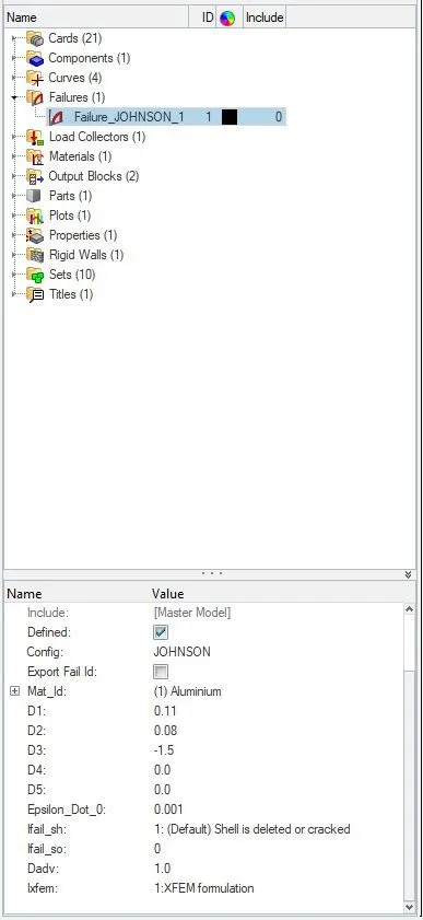
Figure 11: Recommended values provided to the Failure_JOHNSON card, to see the crack in the element.

If Ixfem is equal to 1, it means it is activated. Activating Ixfem leads to element cracking. Fig. 12 shows the rupturing of the aluminum plate, similar to case 2.

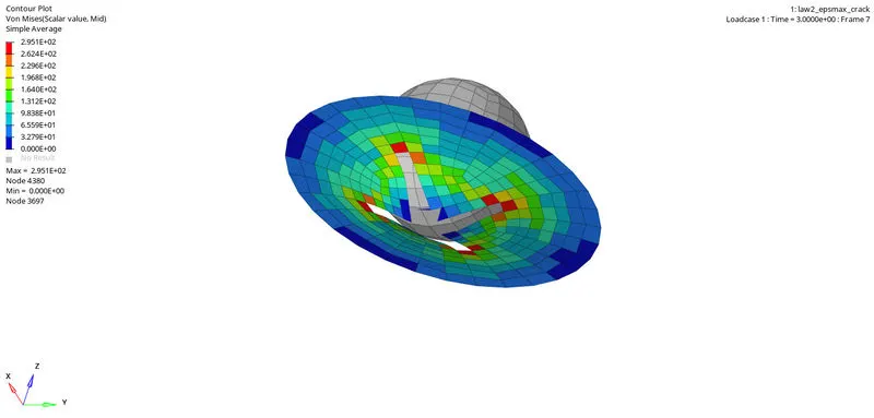
Figure 12: Simulation of the model with law 2 material card image, with Ixfem activated.

The only difference in case 3 is that the failed elements are not completely deleted, however, they are cracking. In fig. 12 cracking of the elements can be observed.

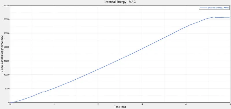
Figure 13: Internal energy vs. time plot for case 3.

The behavior of internal energy is very similar to case 2. However, in case 3, it kept increasing till 4.5 ms. Once there are no elements in contact with the ball, there is no change in internal energy that can be seen because the failed elements had already been cracked.

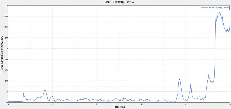
Figure 14: Kinetic energy vs. time plot for case 3.

The kinetic energy is negligible until the elements started failing. Once the elements started failing, some of them disconnected and threw out of mesh with some velocity. This increases the kinetic energy which can be seen in fig. 14, after 3.8 or 3.9 ms.

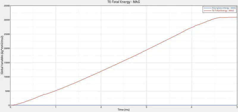
Figure 15: Total energy, and hourglass energy vs. time plot for case 3.

The value of kinetic energy is very small as compared to the internal energy, and therefore the total energy is the replica of the internal energy itself.

CASE 4: No failure card

Johnson-cook material model is used when it is certain that material would fail, or it would undergo plastic deformation. And to see the mode of failure, a failure card is provided, mentioning all the recommended values. In case 4, it was tried to see what happens when law 2 material card is provided with no failure card is provided.

To perform the simulation, the failure was deleted, saved the model, and then run the simulation.

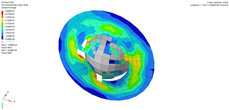
Figure 16: Simulation of the model with law 2 material card image, with no failure card.

When the VonMises stresses for case 4 are observed, it is found that the elements undergone plastic deformation pretty early, and the aluminum sheet was torn apart before 4 ms. The same thing can be observed in fig. 17, the plot of internal energy vs. time.

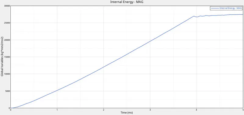
Figure 17: Internal energy vs. time plot for case 4.

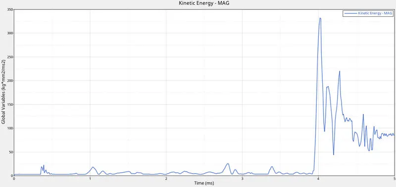
Figure 18: Kinetic energy vs. time plot for case 4.

The kinetic energy was more stable until the aluminum sheet was torn apart at 4 ms, as compared to the other 3 cases. The total energy is again the replica of internal energy, as kinetic energy is negligible. The hourglass energy is zero because of improved shell element properties.

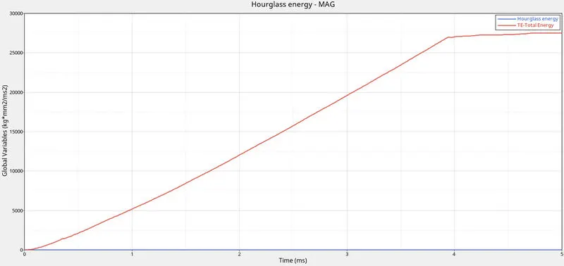
Figure 19: Total energy, and hourglass energy vs. time plot for case 4.

CASE 5: Deleting the value of EPS_p_max

EPS_p_max is the limit of the maximum strain value. If this value is breached by any element, it got deleted. Now, keeping this value equal to zero means that now the element can undergo infinite strain value.

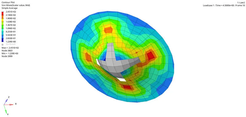
Figure 20: Simulation of the model with law 2 material card image, with no EPS_p_max value.

In fig. 20, it can be observed that the elements are experiencing the stresses, but none of them are getting deleted. It is because the maximum value of stress is kept equal to 425 and the EPS-p_max equal to 0.0.

Figure 21: Internal energy vs. time plot for case 5.

Figure 22: Kinetic energy vs. time plot for case 5.

Figure 23: Total energy, and hourglass energy vs. time plot for case 5.

The internal energy, kinetic energy, and total energy remained the same as in case 4. One significant difference between case 3, case 4, and case 5 is that when Ixfem is introduced in case 3, it dissipated a little more energy than case 4 and case 5. Also, there was more energy error in case 3, as compared to the other two.

CASE 6: Law 27 (PLAS_BRIT)

Law 27 combines an isotropic elastoplastic model with orthographic brittle failure. Using this material model, the plastic zone is lesser than the Johnson-Cook model. The material damage is accounted for before failure. This pre-accounting causes local damage to the material, which further leads to tension and ultimately causes failure in the model. Fig. 24 shows the mode of failure using the PLAS_BRIT model.

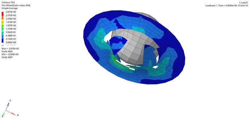
Figure 24: Simulation of the model with law 27 material card image.

The interpretation of the plot of internal energy vs. time for the plas_brit is pretty similar to earlier cases. However, the PLAS_BRIT model stored litter higher energy than the earlier cases, except case 1 (/MAT/ELAST/). And even after breaking, it is further increasing unlike the other earlier cases, which were constant after breaking, This is because two pieces were broken at 4.2 ms, but some pieces were still in contact with the ball, and storing the energy.

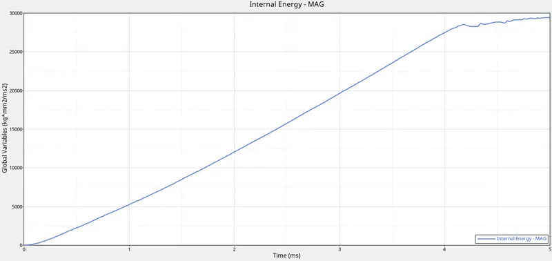
Figure 25: Internal energy vs. time plot for case 6.

The kinetic energy started increasing when the sheet was broken into pieces, and the pieces achieved some velocity,

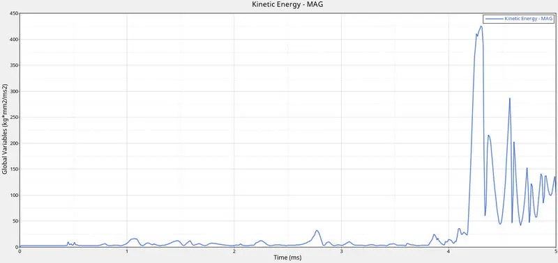
Figure 26: Kinetic energy vs. time plot for case 6.

The total energy is representing none other than internal energy only. It is because the value of kinetic energy is comparably very less than internal energy.

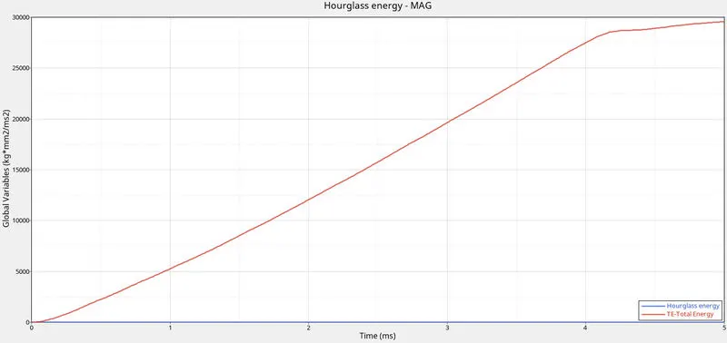
Figure 27: Total energy, and hourglass energy vs. time plot for case 6.

CASE 7: LAW 36 (PLAS_TAB)

This law models an elastic-plastic material using a user-defined function. Practically, it is difficult to determine the material deformation that’s undergoing at different strain-rate and loading. This law allows to provide it with different strain rate values, and then it performs accordingly. Additionally, the johnson-cook failure card can be added with this material model.

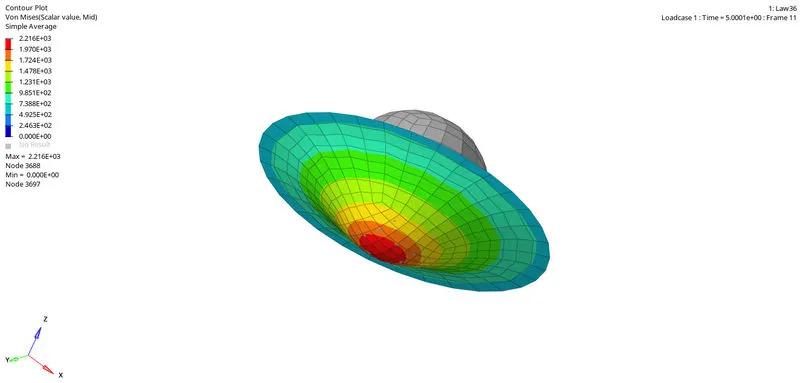
Figure 28: Simulation of the model with law 36 material card image.

The figure showing the mode of deformation with the PLAS_TAB material model. The mode of deformation is quite similar to the ELAST material mode (case 1). It might be because enough values are not provided, and the EPS_p_max value is not getting reached. The energy error is acceptable, but still greater than other cases, except case 3.

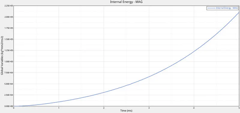
Figure 29: Internal energy vs. time plot for case 7.

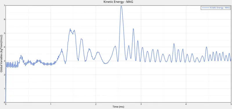
Figure 30: Kinetic energy vs. time plot for case 7.

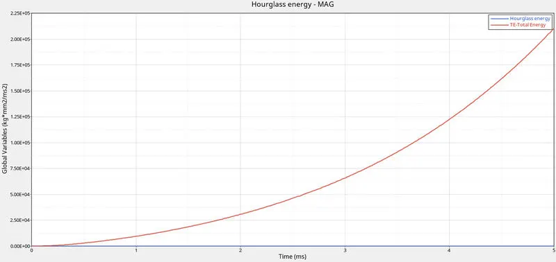
Figure 31: Total energy, and hourglass energy vs. time plot for case 7.

Observing the internal energy, and total energy of case 7 and case 1, it can be said that the aluminum sheet is undergoing elastic deformation. And because the strain is not reaching the EPS_p_max value, no elements are deleting and the graph is not showing any change in its pattern, after its one consistent parabolic pattern, like it was observed in case 2, case 3, case 4, case 5, and case 6.

RESULT AND DISCUSSION

There were 7 cases to analyze. Each case had a difference in its material model. In case 1, the material was modeled with the elastic material model. The law 1 or /MAT/ELAST/ model works in the linear elastic region of the material, and therefore, failure in the material cannot be observed. Although, if the value of stress is going beyond the yield strength value, it should be considered that the material is undergoing plastic deformation, and therefore, it should be analyzed with law 2, or law 36. Because the material acts in a linear elastic region, the energy dissipation with this law is not proper, and therefore this law must be used only in the case where the applied load will not deform the material beyond the yield stress value.

In case 2, case 3, case 4, and case 5 the material was modeled with law 2 or the Johnson-Cook material model. Some slight changes were made in each case to see which mode of failure is more realistic. Case 2 was defined with EPS_p_max value, which is the maximum strain value. If this strain value is crossed, the element deletes. However, the element deletion is seemed to be not so realistic. Therefore, in case 3 Ixfem is introduced, which is when activated, the element cracking becomes possible, and therefore, it gives a much more realistic view of the circumstance. But, using Ixfem, the energy error increases, and therefore it must be used whenever necessary. The more energy error using Ixfem is proof that the energy dissipation is not convenient, and therefore the max. VonMises stress value is also increased.

In case 4 and case 5, when the failure card is deleted, and EPS_p_max value is deleted respectively, there is no difference concerning case 2. However, in case 4 the plastic deformation has started pretty early than case 2, and the element does not delete in case 5.

In case 6, the law 27 or /MAT/PLAS_BRIT/ material model was used. This model narrows the plastic region. It stores the energy at the local level, further causing tension in the element and ultimately the failure. Because of energy storage, the stress value also increases, and therefore elements break with high velocity, which leads to a sudden increase in the value of kinetic energy.

Practically, when some accidents occur, the material deformation does not occur at the same strain rate value. So, to get the on-site results, the PLAS_TAB material model was used, which was provided with the value of different strain-rate values. Generally, the more the value of strain-rate more early would be the failure. In case 7, this model showed the behavior like case 1 (/MAT/ELAST/). It is because the strain value did not reach EPS_p_max value, and thus acted like an elastic model. Moreover, it stored much energy, and therefore, the stress value increased.

	Description	Total Number of Cycles	Energy Error	Mass Error	Simulation Time	Max. VonMises Stress
CASE 1	Law 1 (/MAT/ELAST/)	47968	1.3%	0.000	54.27 s	1.433E+03
CASE 2	Law 2 (EPS_p_max failure)	49379	0.8%	0.000	54.88 s	2.752E+02
CASE 3	Law 2 (Ixfem = 1)	49216	4.1%	0.000	56.28 s	2.559E+02
CASE 4	Law 2 (No failure card)	49407	0.8%	0.000	54.81 s	2.707E+02
CASE 5	Law 2 (No EPS_p_max)	49303	1.1%	0.000	54.71 s	2.451E+02
CASE 6	Law 27 (/MAT/PLAS_BRIT/)	49506	0.8%	0.000	56.43 s	2.875E+02
CASE 7	LAW 36 (/MAT/PLAS_TAB/)	39517	3.7%	0.000	44.48 s	2.216E+03

CONCLUSION

Case 1 is about the Elastic model, which has to be used for the model which would not reach the yield strength value. Case 3 (Ixfem=1) can be used for observing realistic scenarios, but the energy dissipation in it is not so proper. Case 4 (no failure card) shows pretty early plastic deformation, and case 5 (No EPS_p_max value) shows no element deletion. Case 7 is about the brittle nature of the model, which is not recommended for a ductile material. Therefore, the only material models which could give a realistic view of the circumstance are case 2 (law 2 with defining the value of EPS_p_max_, and case 7 (PLAS_TAB).