Assignment 4-RADIOSS Material Laws Challenge

Aim

To run crash analysis on the given model by applying different materials laws available in Radioss and post-process the results

Objective

To carry out simulations of the given starter files and compare the results. There shall be 7 cases (according to given parameters) and they are to be compared primarily via animations and plots. The files to be worked on are the FAILURE_JOHNSON_0000.rad file and the LAW27_0000.rad file. The cases are as follows:

• Law 2 (file: FAILURE_JOHNSON_0000.rad) - base simulation.
• Law 2 (file: FAILURE_JOHNSON_0000.rad) with Ifail_sh = 1, Dadv = 1, and Ixfem = 1.
• Law 2 (file: starter file for case 2) with fail/JOHNSON card deleted.
• Law 2 (file: starter file for case 3) with EPS_p_max value deleted
• Law 1 (file: FAILURE_JOHNSON_0000.rad) with fail/JOHNSON card deleted and values for density, E, nu assigned
• Law 27 (file: LAW27_0000.rad) with recommended shell properties
• Law 36 (file: LAW27_0000.rad) with recommended shell properties and given reference curve.

Theory

The accuracy of the simulation depends on the material chosen.Choosing the right material and providing the reliable material data in performing a simulation is very important.RADIOSS has multiple material properties and wide variety of material library like concrete, foam, rubber, composites etc.,

Some of the commercially used material laws are:

• Law 1: Elastic (Isotropic Elasticity)
• Law 2: Johnson-cook (Isotropic Elasto-plastic)
• Law 27: Elastic-plastic brittle
• Law 36: Elastic-plastic tabulated
• Law 42: Ogden (visco hyperelastic)
• Law 70: Foam

Isotropic Elasticity - Law 1

Isotropic means that a material will have the same material properties in all 3 directions. Under isotropic elasticity, RADIOSS provides two types of elasticity.

• Linear elastic: LAW1 elastic
• Hyperelastic: LAW69 Tabulated hyperelastic, LAW82 Ogden
• The RADIOSS elasticity law follows the hook’s law of elasticity i.e a linear relationship between the stress and starin.
• It is available for truss, beam, shell, and solid elements.
• As mentioned earlier, it is exclusively for elastic materials.
• The material stiffness is determined by Young’s modules of elasticity (E) and Poisson’s ratio (n).
• The sheer modulus G is calculated by [Math Processing Error]

Limitations

Elastic materials cannot be used for large deformation cases such as blow molding etc. In the case of large deformation, law 2 johnson-cook material with high yield can be used.

Isotropic Elasto-Plastic

RADIOSS provides various types of elasto-plastic material laws. It has all the material models based on von mises hardening without damage, von mises hardening with ductile damage, von mises with visco-plastic flow.Here, we are going to look at Johnson-cook/JOHNS and tabulated piece-wise linear/PLAS_TAB.

(PLAS_JOHNS) Johnson-cook material- Law 2

This law represents an isotropic elasto-plastic material using the johnson-cook material model.The model expresses material stress as a function of strain, strain rate, and temperature.In the material card, we have an option called EPS_max which is nothing but plastic strain at failure. Failure of the element happens when 1 integration point reaches EPS_max.Now if failure is only based on EPS_max, there can be instances where the EPS_max gives out unrealistic results. To avoid this, we have the option called /FAILS/JOHN./FAIL/JOHN card provides the user with more control over the failure of the johnson-cook strain.

LAW36-PLAS_TAB Elastic plastic piecewise linear material

The LAW36 material law helps in modelling isotropic elasto-plastic material using user defined functions for the work hardening portion of the stress-strain curve for different strain rates.The curve defined is nothing but the stress-strain curve after the yield point. The yield point is set to 0.This material law is available for both brick and shell elements.If the work hardening portion is defined by the user, then its elastic portion is taken from the inputted young’s modulus and poisson’s ratio.Any number of stress-strain curves can be defined.The important part is that the strain rate curves must not intersect with each otherThe plastic strain curve should start with 0.The user also has option to input yield stress with respect to pressure using fct_Idp.

Procedure

Case 1

Import the FAILURE_JOHNSON_0000.rad file and run the model as it is. Give the title name as Law2_epsmax_failure.

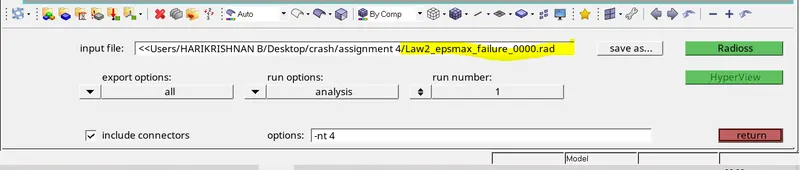
To run the simulation, Go to Analysis >> Radioss. We need to save the output files in a new folder so that we can access them easily. The file is saved as "Law2_epsmax_failure_0000.rad". After saving, tick the 'include connectors' box and type in '-nt 4' in the options text box as shown below, before clicking 'Radioss'
It is recommended to be written as "-nt 4" as shown in the image below. This means assigning the task to 4 cores in the system, to perform the simulation faster. It depends upon the process of our computer (it has a quad-core processor, then it should be taken as 4. If the system has an octa-core processor, then it is taken as 8). And "nt" means "number of threads". Then click on "Radioss", in order to run the simulation

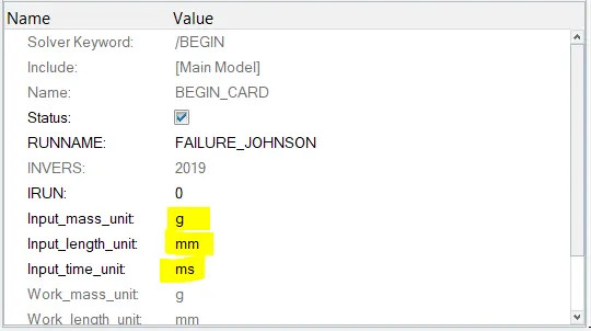
By clicking 'Radioss', we get the solver window as shown below, which basically tells us what the RADIOSS solver is doing. After a few minutes, radios does the job and you can check all the files in the folder which you have saved as.

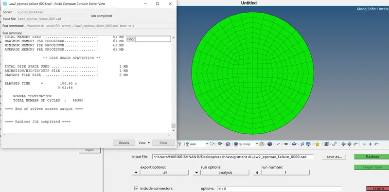
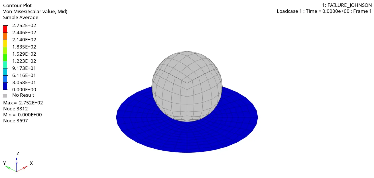
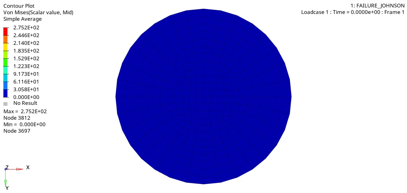
The simulation is complete, now we just need to visualize it. For that, we need to switch to the Hyperview utility.After accessing Hyperview, we should input the simulation file. For this, use h3d file that was generated when RADIOSS processed the starter file. It is generated in the files swhich are shown in the picture above. After selecting it, we can click 'apply'.After accessing Hyperview, we are asked to input the simulation file. For this, we shall be using the h3d file that was generated when RADIOSS processed the starter file (Law2_epsmax_failure.h3d). It should be generated in the same folder. After selecting it, we can click 'apply'. Doing so generates the simulation animationWe can change what is being represented by selecting the 'contour' option in the toolbar. In this case, we can change the result type to 'Von Mises' and change the averaging method to simple. Doing so creates the Von Mises stress contours as shown below.

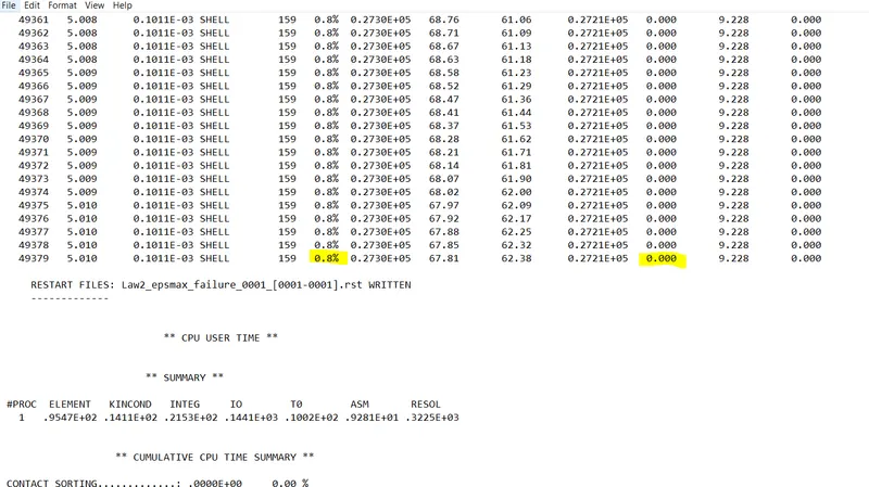
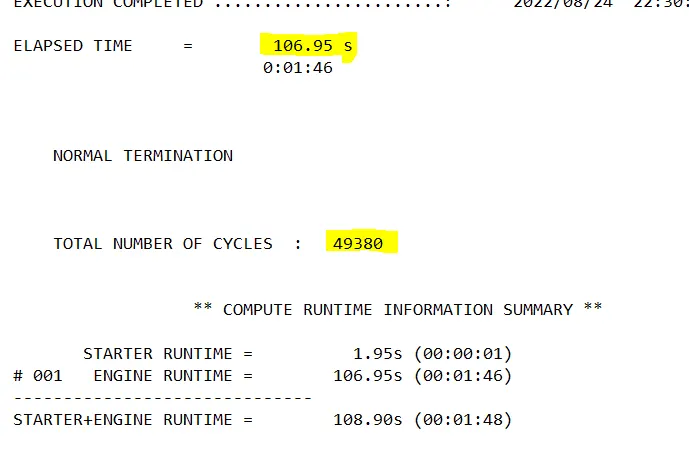
Next step is to carry out energy error and mass error checks and this is done by analyzing the RADIOSS engine output file. This can be accessed from the same directory as the starter and engine files and is denoted by the '.out' extension. We need to check the file that contains '_0001.out' by using any text editor.On opening the file and scrolling down to the end, we can see the final energy and mass error values.The final energy error is 0.8%, which is very acceptable. The closer to 0 it is, the better and there is no mass error. Overall, these are very good values.

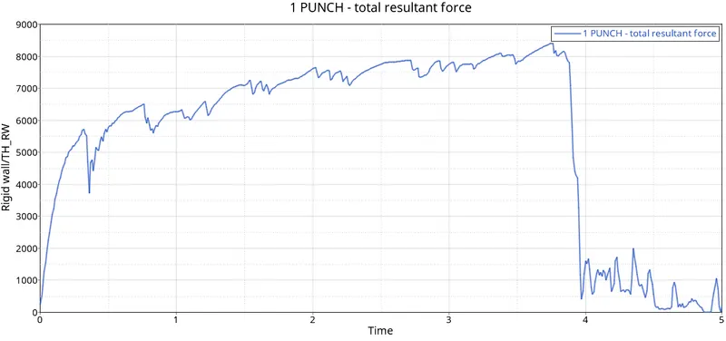
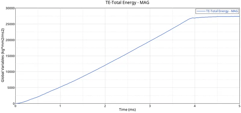
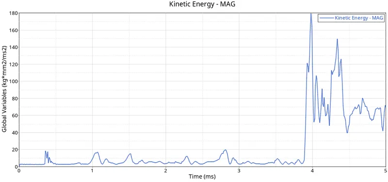
Now plot the graphs in Hypergraph 2D. We can switch to it using the same client selector option in the toolbar.In the Hypergraph section, we need to input a file. For this, we will be using the result file generated by the RADIOSS solver (also known as the 'T01 file'). This file is available in the same directory as the starter, engine, and animation files. The file name ends with 'T01'.

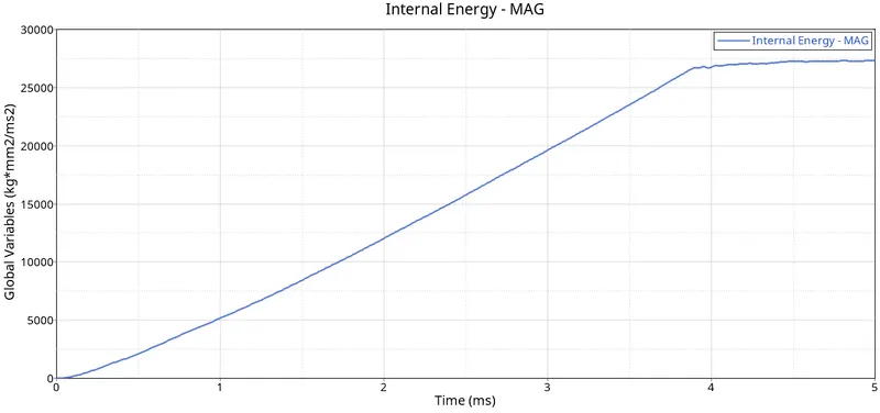
The graph plotted

Case 2

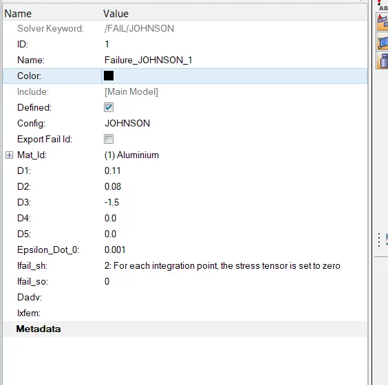
• Import the case 1 rad file, named “Law2_epsmax_failure” and perform the simulation with failure plastic strain (EPS_p_max) and fail_Johson card enabled.
• Changes to be made in /FAIL/JOHNSON card:
• ifail_sh= 1
• Dadv= 1
• Ixfem= 1
• Use the recommended values for the property card.
• Give the title name as Law2_epsmax_crack.

1. Ifail = 1,which determines the Shell element Failure method. So there are two ways in which we can see the element failing, the element will either get deleted or in some cases the cracking occurs according to the material properties.
2. Ixfem: In this, we can choose that if there is any element that is failing we want that element to delete or we want the element to be crack.We are going to take Ixfem=1. Which allow failed element to cracked not to delete.
3. Dadv :It gets activated when we have taken Ixfem=1. We are going to takeDadv=1. Which gives the criteria that how much an element can get break into small pieces. If it goes beyond the limit the element gets delete.

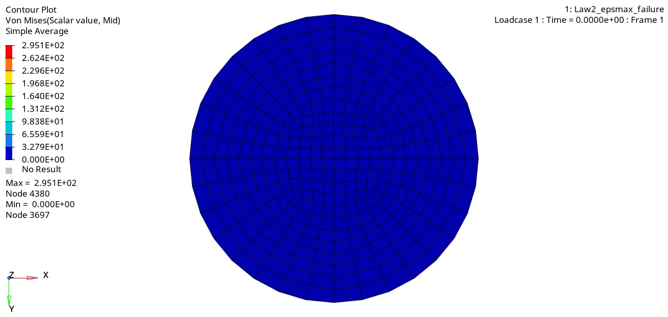
Now run the analysis and the file is saved as “Law2_epsmax_crack_0000.rad”. With connectors ticked and '-nt 4' typed in the options box, we can click the Radioss button to run the analysis.After the solver window completes the analysis, as usual, switch to HyperView window and run the h3d file of the current analysis - Law2_epsmax_crack.h3d and set the Von Mises stress contours:

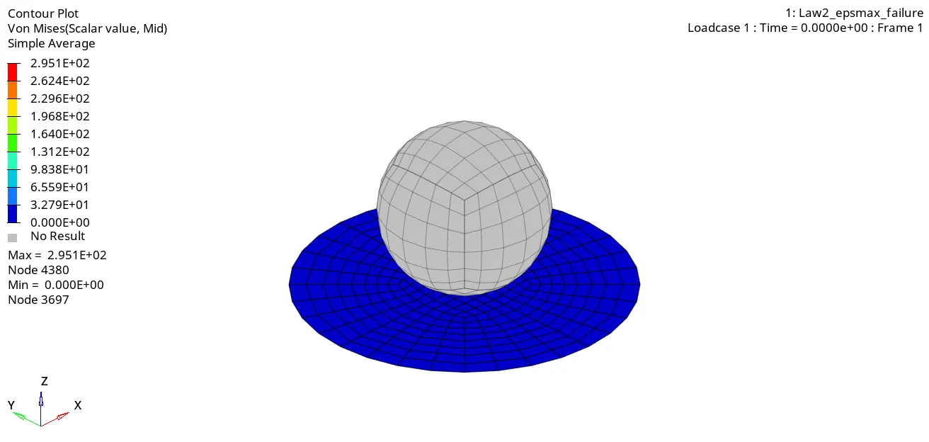
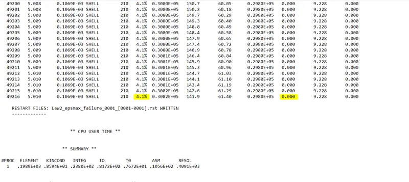
Now, check the energy and mass error on the RADIOSS output file Law2_epsmax_crack_0001.out. The energy error is decent enough and is lesser than 5% and mass error is non-existent. We can go ahead and switch to Hypergraph to plot the graphs.

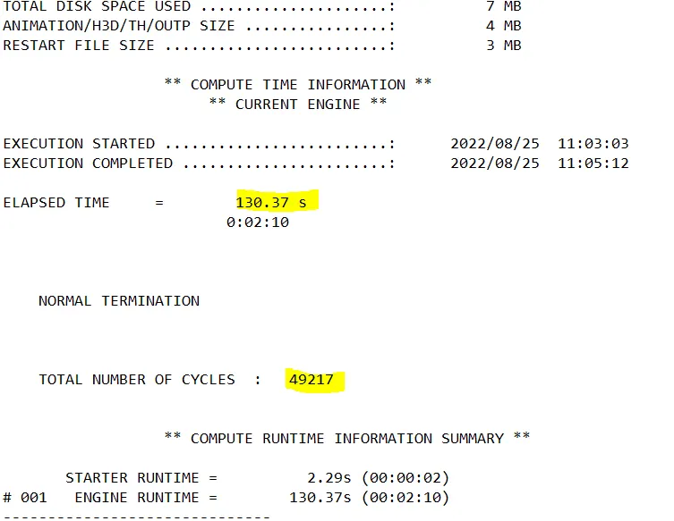
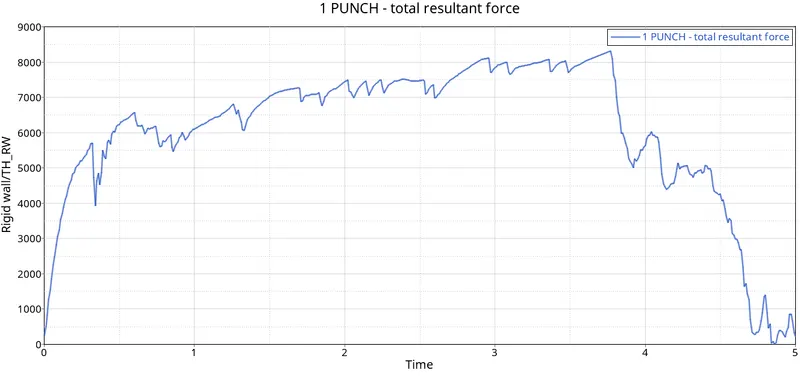
The graph plotted

Case 3

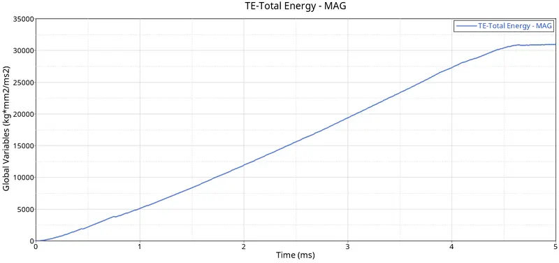
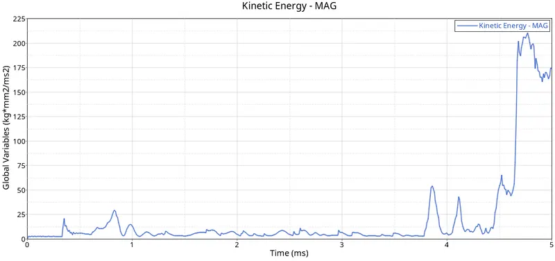
Import the case 2 rad file, named “Law2_epsmax_crack” and perform the simulation by removing the fail_Johnson failure card. Give the title name as Law2_epsmax_nofail.

Again, we need to switch to Hyper works and import the solver deck file “Law2_epsmax_crack_0000.rad”, the starter file created in the previous case.In this case delete the fail/JOHNSON card. Go to Failures > Failure_JOHNSON_1.

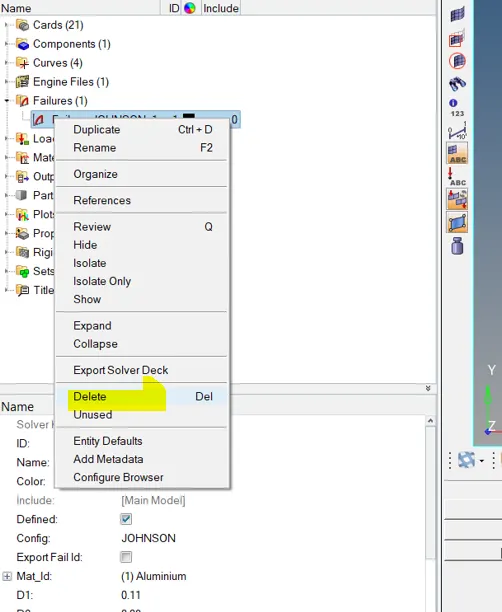
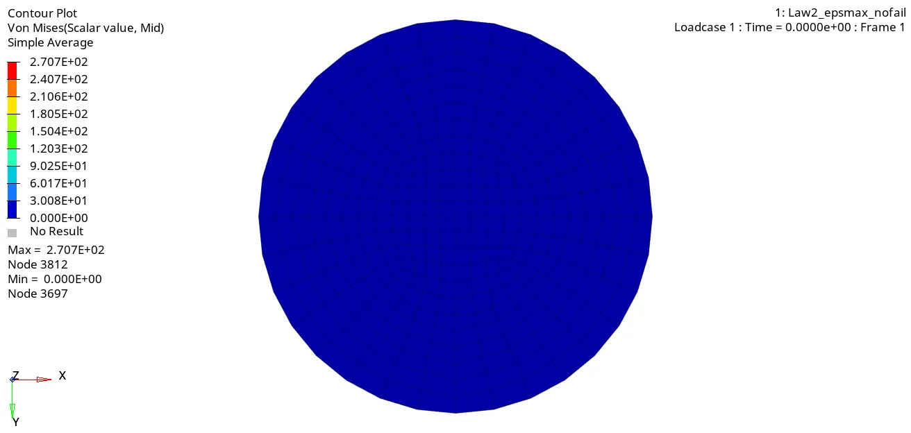
Now run the analysis and the file is saved as “Law2_epsmax_nofail_0000.rad”. With connectors ticked and '-nt 4' typed in the options box, we can click the Radioss button to run the analysis.After the solver window completes the analysis, as usual, switch to HyperView window and run the h3d file of the current analysis - Law2_epsmax_nofail.h3d and set the Von Mises stress contours.

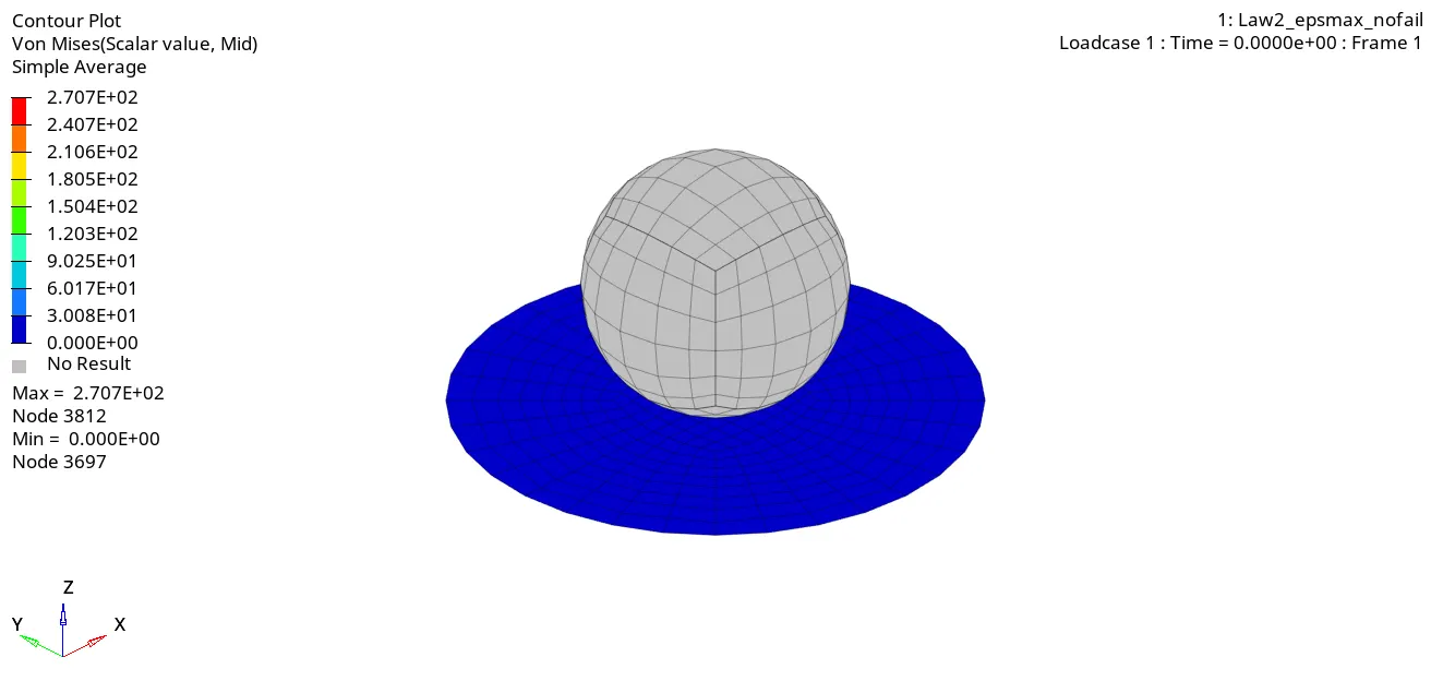
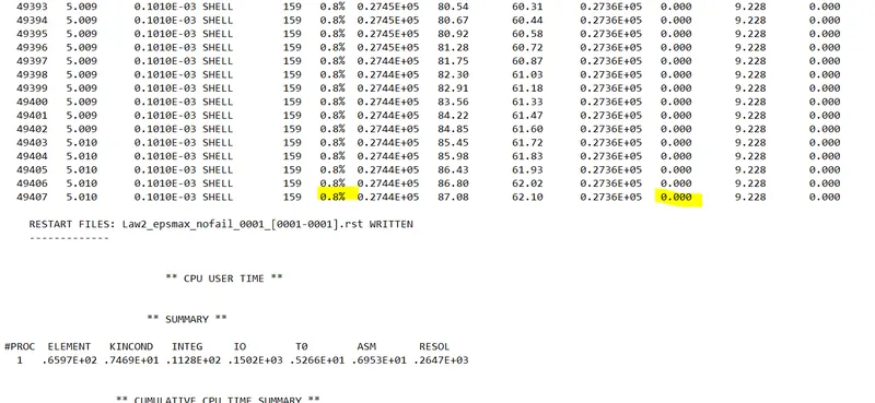
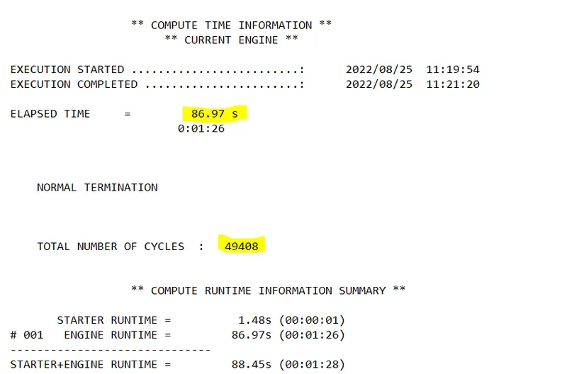
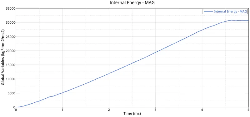
Now, check the energy and mass error on the RADIOSS output file Law2_epsmax_nofail_0001.out. The energy error is almost 0 and the mass error is non-existent. Now we can switch to Hypergraph to plot the graphs.

The graph plotted

Case 4

Import the case 3 rad file, named “Law2_epsmax_nofail” and perform the simulation by removing both the failure plastic strain (EPS_p_max) and the fail_Jhonson failure card.

In this case, import the case 3 starter file - Law2_epsmax_nofail_0000.rad.This time, delete the EPS_p_max value (make it as 0). Going to the model tab, we can go to Materials > Aluminium as shown below.

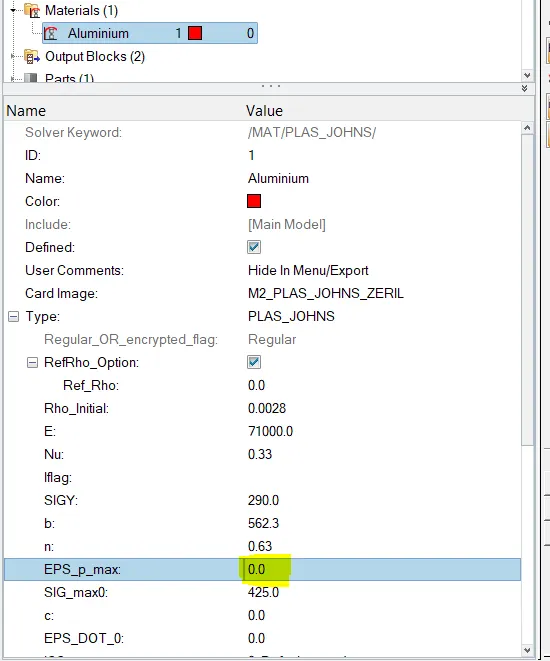
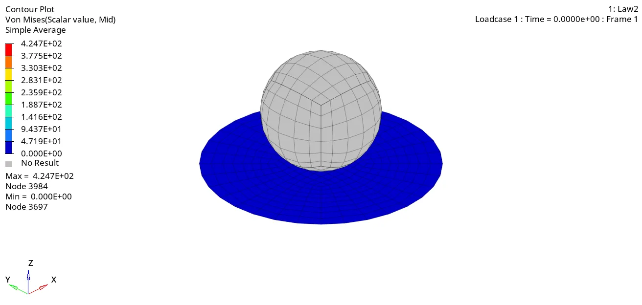
After that, we can switch to the Radioss analysis section via Analysis > Radioss, save the file as 'Law2_0000.rad', enable connectors and type in '-nt 4' in the options section and run the analysis by clicking 'Radioss'.After the solver finishes its analysis, we can switch to Hyperview, run “Law2.h3d”, activate the Von Mises contours and view the simulation

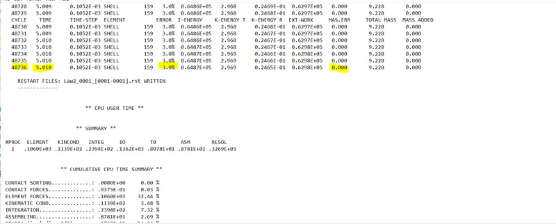
Now, check the energy and mass errors on “Law2_0001.out”. The energy error is less than 5% and mass error is non-existent.

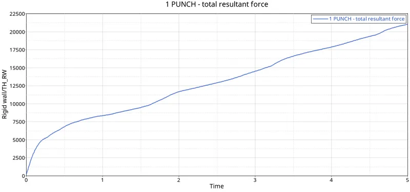
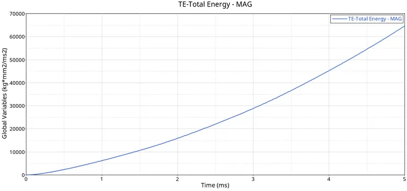
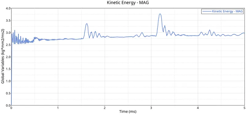
The graph plotted

Case 5

Import the case 4 rad file and perform the simulation by changing the material card to Law 1. Keep the same value for rho, E, and nu values.

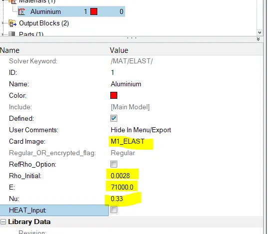
In this case import the main starter file - Law2_0000.rad. After that, go to Materials card > Aluminium and change the card image to M1_ELAST, which is Law 1.Also set the values for Rho_Initial, E & Nu as follows:
Rho_initial = 0.0028, E = 71000.00, nu = 0.33.

Now do the analysis and save the file as “Law1_0000.rad”. Just as before, enable connectors and type '-nt 4' in the options box. Then, we can click radioss and let the solver run the analysis. After the solver completes the analysis, we can switch to Hyperview, import the 'Law1.h3d' file, enable the Von Mises contours and view the simulation:

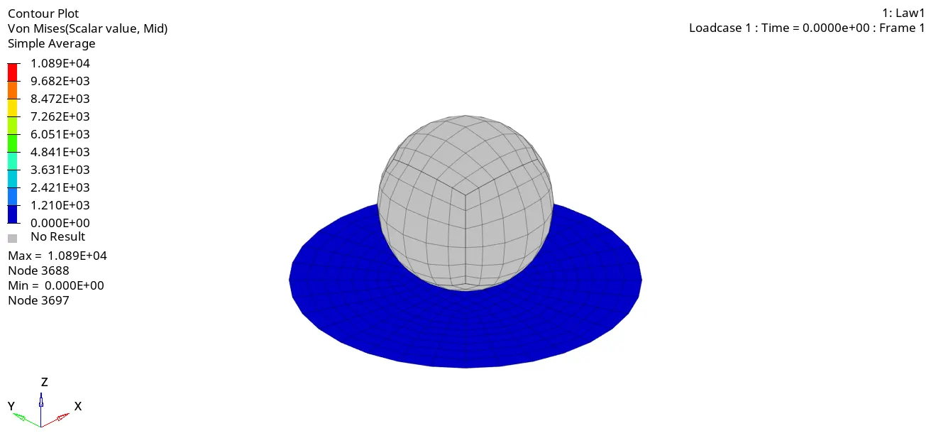
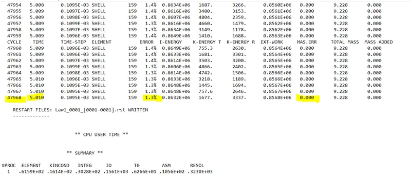
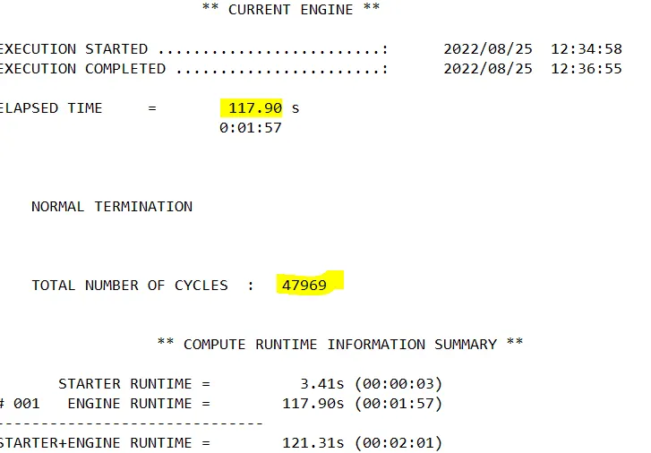
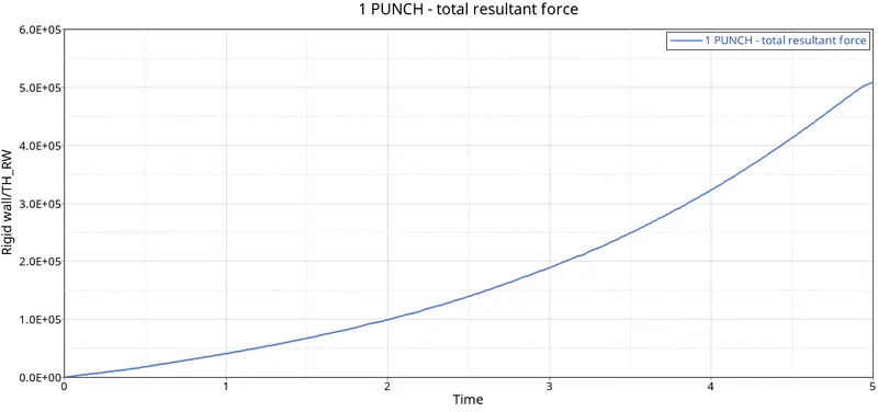
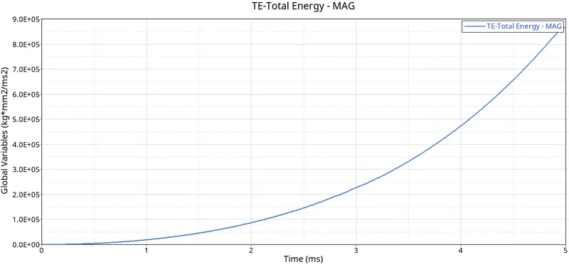
Now, check the energy and mass error on the RADIOSS output file Law1_0001.out. The energy error is less than 5% and the mass error is non-existent. We can then switch to Hypergraph to plot the graphs for this simulation.

The graph plotted

Case 5

Import the case 4 rad file and perform the simulation by changing the material card to Law 1. Keep the same value for rho, E, and nu values.

Import the case 1 rad file, named “Law2_epsmax_failure” and Go to the model tab and here, we shall be creating a new curve (as per instructions given in the week-4, Materials 7 video). Right-Click >> Create >> Curve. Initially, there are 4 curves, we are adding the new curve named CASE7.

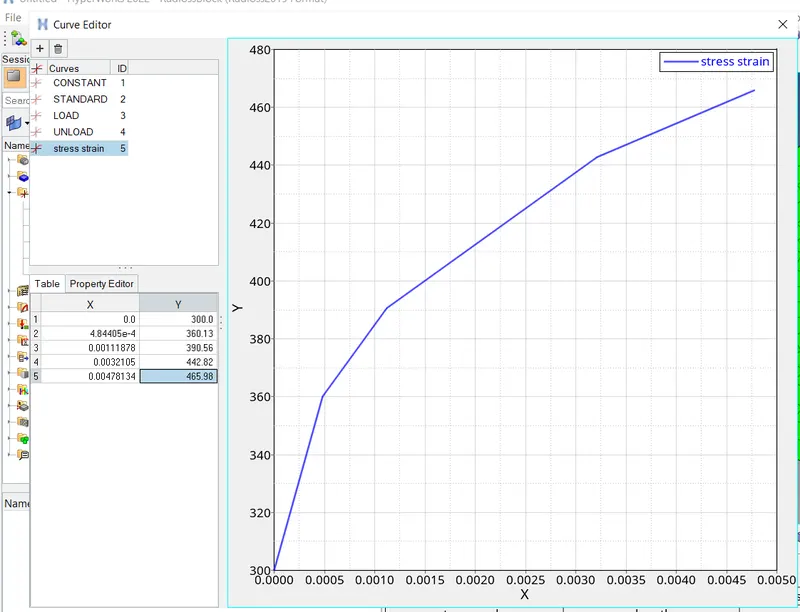
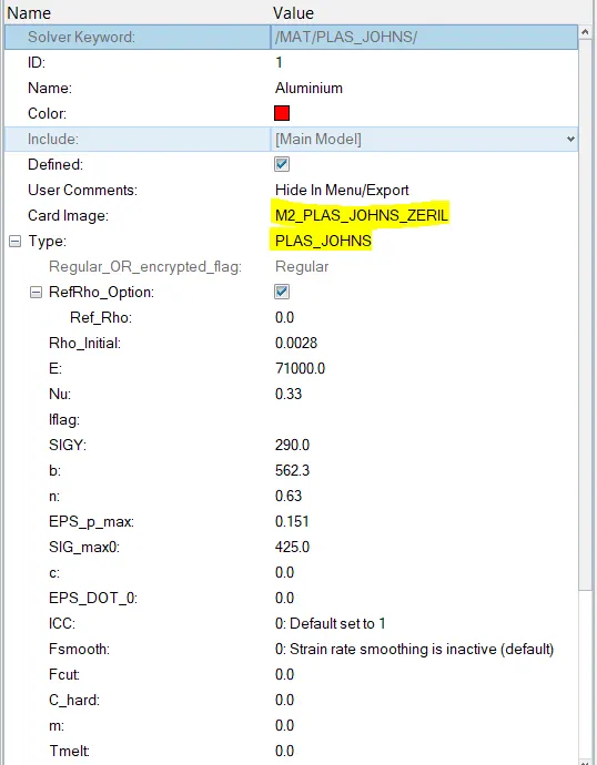
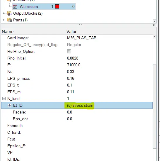
Now go to Materials >> Aluminium and change the card to M36_PLAS_TAB (Law 36). After that, set the values for Rho_Initial, E & Nu as follows:
Rho_initial = 0.0027, E = 71000.00, nu = 0.33. We can then add the curve using the N_funct attribute. We can change its value to 1 and by doing so, it lets us select the reference curve. We shall select the one we just made.

Now run the analysis using the Radioss tool via Analysis > Radioss. The same process, as in previous cases, is repeated. This time, we shall name the file “LAW36_0000.rad”. After the analysis is complete, we can switch to Hyperview and import 'LAW36.h3d'. With Von Mises contours enabled, we can view the simulation.

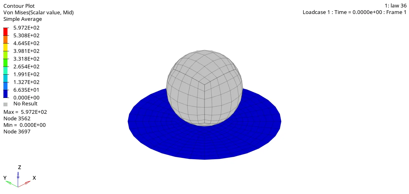
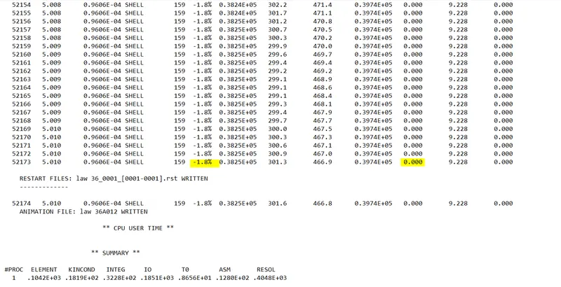
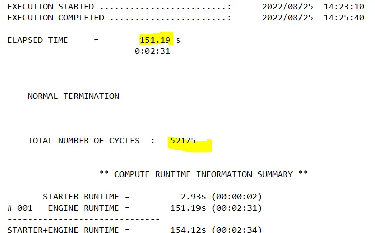
An energy error of -1.1% is very acceptable since it's very close to 0. As usual, the mass error is non-existent. Now we can switch to Hypergraph to plot the graph for this simulation.

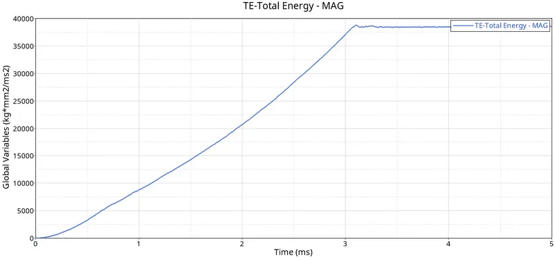
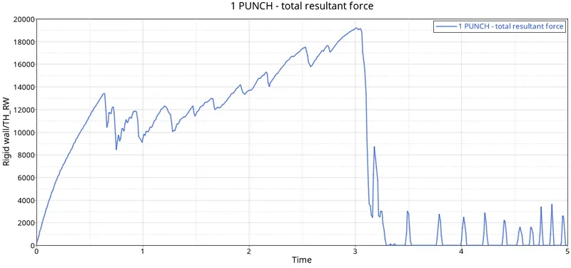
The graph plotted

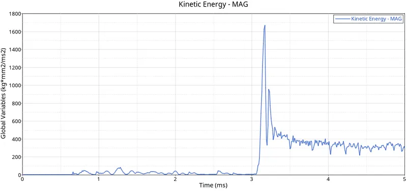
Case 7

Open the Law27_0000.rad file and perform the simulation with the law 27 material card. Use the recommended shell properties.

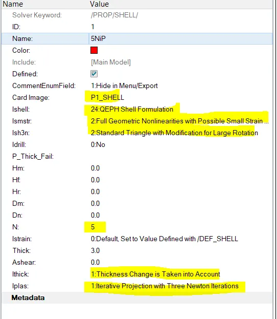
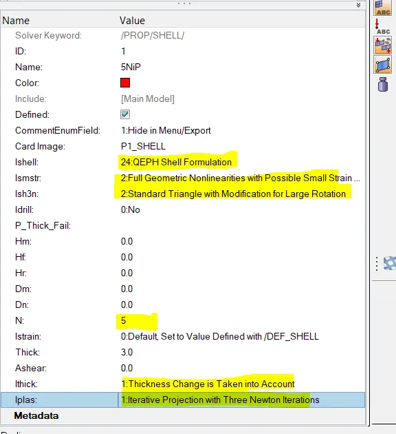
In this case, import the 'LAW27_0000.rad' file. We need to use recommended shell properties in this case. Go to Properties > 5NiP. Now, we can look at the utility window and set the following attributes as follows:

I_shell=24, I_smstr=2, I_sh3n=2, N=5, I_thick=1, I_plas=1

Now, run the analysis via the Radioss tool. This time, we can save the file as 'Law27_0000.rad'. Just as before, we can enable connectors and type '-nt 4' in the options box. Then, we can click radioss and let the solver run the analysis. After it's done, we can generate the simulation via Hyperview with the Von Mises contours enabled as shown.

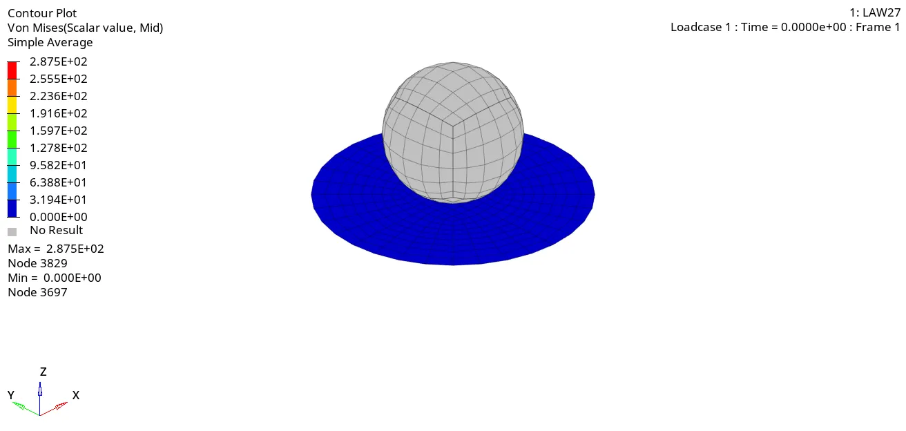
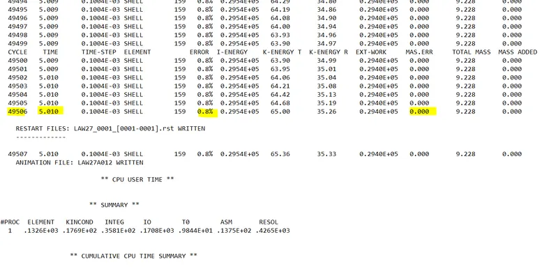
we can check the energy and mass errors on “Law27_0001.out”. The energy error is very close to 0 and the mass error is non-existent.

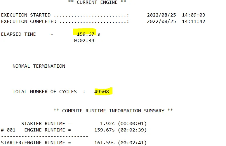
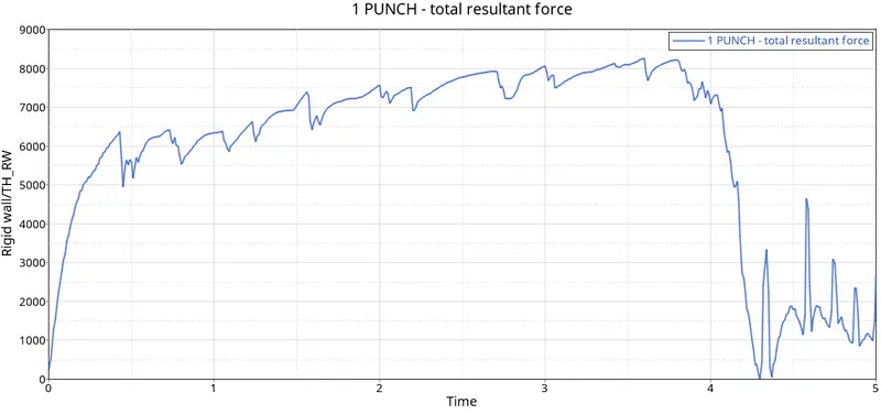
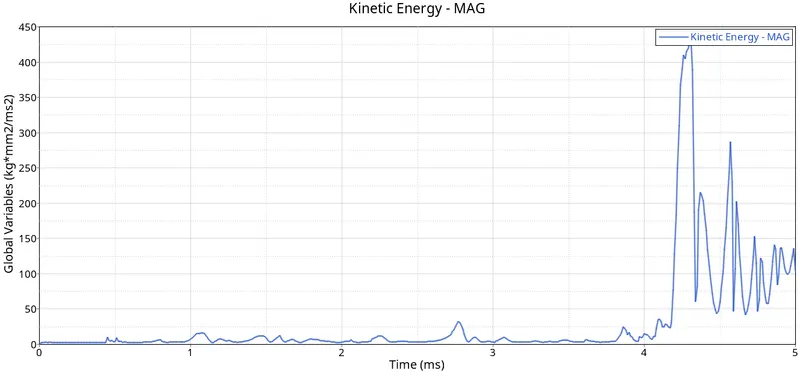
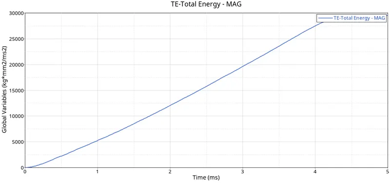
The graph plotted

OBSERVATION

The energy graph and the Von Mises give a great idea and it's very helpful to understand the material card and the behavior accordingly.

Case	Material law	Simulation name	Energy error (%)	Simulation time (s)	Number of cycles	Maximum stress value (MPa)	Element behaviour
1	Law 2 (Johnson-Cook model)	EPS_max_failure	0.8%	106.95	49380	275.2	Deleted
2	Law 2 (Johnson-Cook model)	EPS_max_failure_Crack	4.1%	130.37	49217	295.1	Cracks first then deleted
3	Law 2 (Johnson-Cook model)	EPS_max_nofail	0.8%	86.97	49408	270.7	Deleted
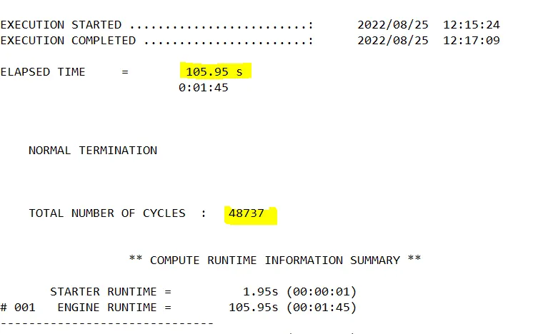
4	Law 2 (Johnson-Cook model)	Law 2	3.0%	105.95	48737	424.7	Preserved
5	Law 1 (linear elastic material)	Law 1	1.3%	117.90	47969	108.9	Preserved
6	Law 36 (elasto-plastic materia)	Law 36	-1.8%	151.19	52175	597.2	Deleted
7	Law 27 ( brittle failure model)	Law 27	0.8%	159.67	49508	287.5	Deleted

CASE 1. Internal Energy graph	CASE 1. Von Mises
CASE 2. Internal Energy graph	CASE 2.Von Mises
CASE 3. Internal Energy graph	CASE 3.Von Mises
CASE 4. Internal Energy graph	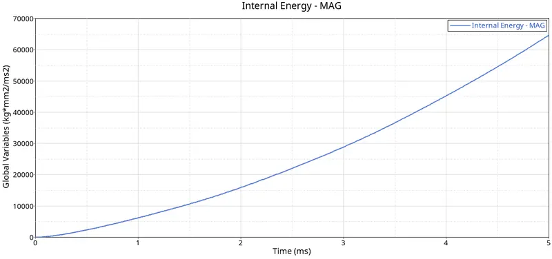CASE 4.Von Mises
CASE 5. Internal Energy graph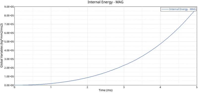	CASE 5.Von Mises
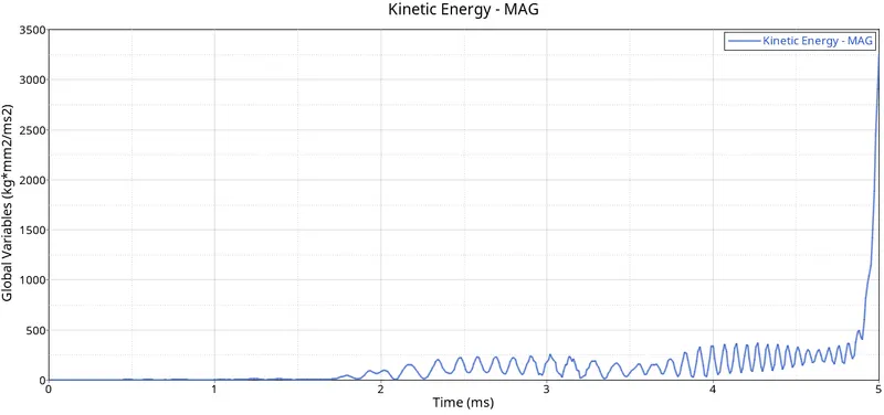
CASE 6. Internal Energy graph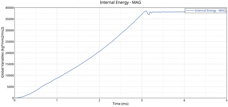	CASE 6.Von Mises
CASE 7. Internal Energy graph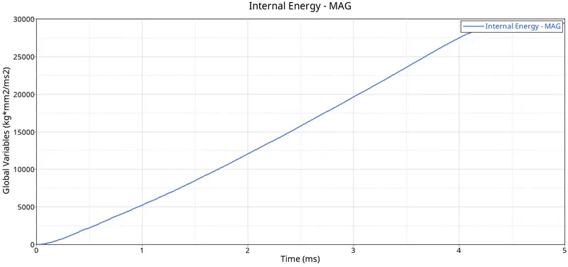	CASE 7.Von Mises

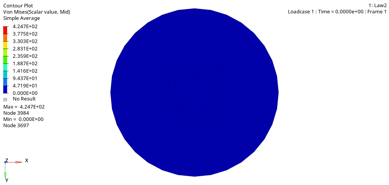
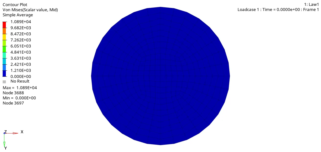
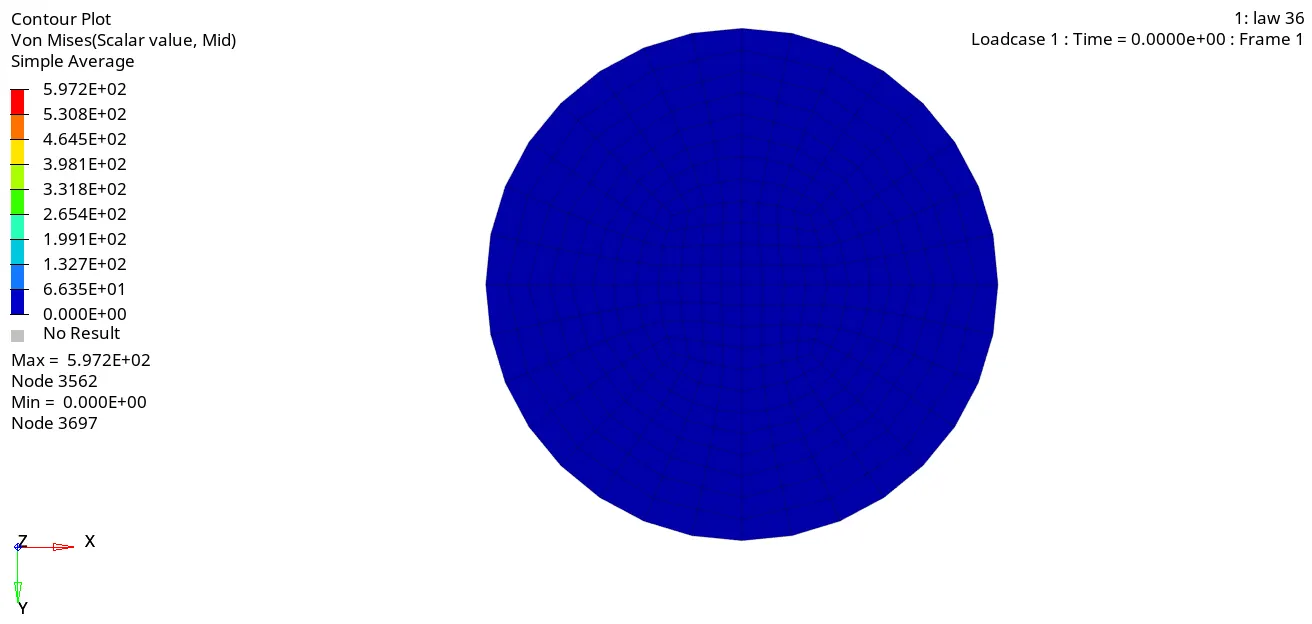
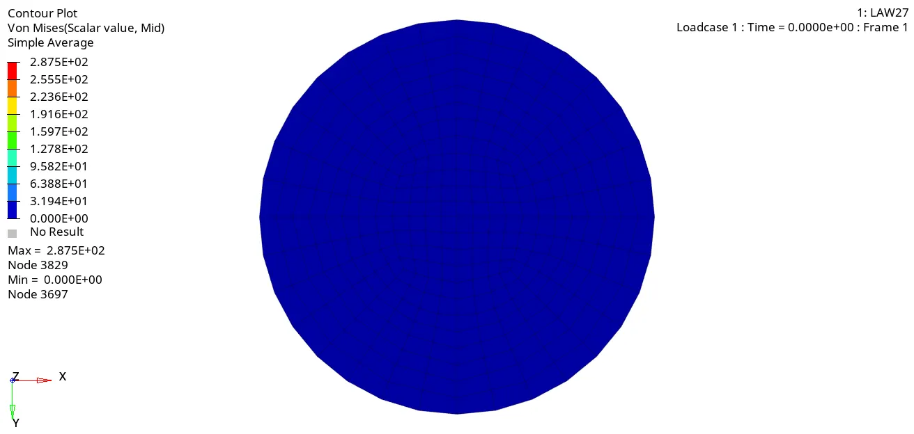
stresses devloped in diefferent material formulation.Based on the stresses developed in the material, and given material data for aluminum with yield stress of 290Mpa and maximum stress of 425MPa, case 2 presentes the on-field scenario compaired to rest of the cases.

Conclusion

Comparison between different material cards and failure cards has been carried out by applying them to the given simulation model. Element behaviour and stress development has been discussed. Based on the observation of results: case 2 presents the best on-field scenario in the simulation.

Selecting a correct material model plays a very important role in simulation. Selecting the wrong material model and doing simulation will also give result but it will not represent the actual situation.

Law 1 is used to model purely elastic materials or materials that remain in the elastic range. To model this we require Poisson's ratio and Young's modulus. This law represents a linear relationship between stress and strain.

Law 2: In this law, the material behaves as linear elastic when equivalent stress is lower than the yield stress. For a higher value of stress, the material behaves like plastic. Failure can be captured better with the help of an optional Fail_Johnson card.

Law 27: Used for brittle materials.

Law 36: The elastic-plastic behavior of isotropic material is modeled with user-defined functions. The stress-strain curve is modeled using E and Poisson's ratio. Therefore, it is the best card because we cannot know the exact failing condition of the material in the other cases, but we can define the stress-strain curve, and then we can decide where the material is failing.