Assignment 4-RADIOSS Material Laws Challenge

Aim: To run the simulation on rupture plate model by using Johnson cook material & elastoplastic material with brittle failure by using RADIOSS.

OBJECTIVE:

1. To run the model as it is with default failure parameters.
2. To run the model by changing given failure parameters.
3. To run the model by deleting failure parameters.
4. To run the model by deleting the value of failure plastic strain(EPS_p_max).
5. To convert the material model to Law1 elastic with same mechanical properties.
6. To run the model by using M27_PLAS_BRIT, change the shell properties to recommended shell properties and Johnson cook parameters but different value for EPS based failure.
7. To run the model by using M36_PLAS_TAB material.
8. To check total number of cycles, energy error, mass error and simulation time for all cases.
9. To plot energies for all cases.

PROCEDURE:

Open the hyperworks software, and then we have to set user profile interface i.e. Optistruct or RADIOSS. Optistruct is implicit solver which handles small deformations. And RADIOSS is explicit solver which handles large deformation. So we will use RADIOSS as user interface.

First we have to import the required file i.e. FAILURE_JOHNSON_0000.

File--->Import---->Solver Deck---->File: select file--->Import.

Once file is imported, model will look like as shown in picture below. A rupture plate is made up of aluminum so it is a deformable body and ball is a rigid body which means it is a non-deformable body.

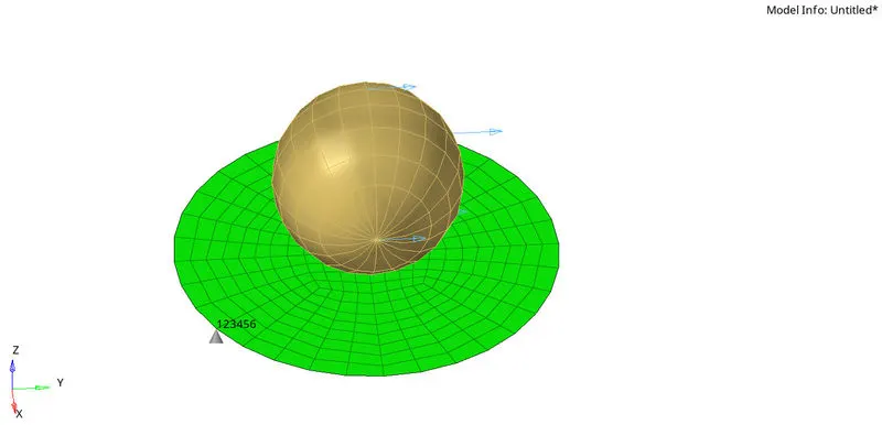
Radioss follows measurements in grams, millisecond and millimeter unit system.

And we are going to use aluminum material but with different card images as per requirement. So in material card default material parameters are as shown in picture below.

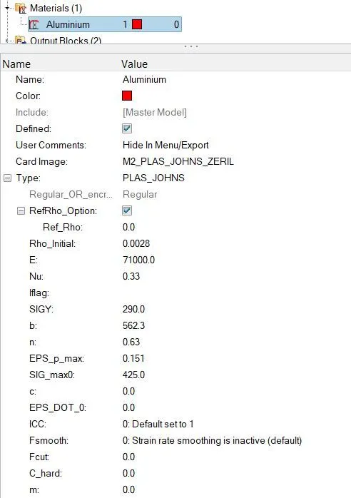
And in property card parameters, we are having elements formulation parameters which are set to be recommended by default as shown in picture below.

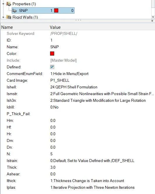
And for all cases we are going to use default termination time and animation time step frequency too.

CASE 1: To run the model as it is with default failure parameters.

For this case, first we have to import the required file i.e. FAILURE_JOHNSON_0000.

As per requirement for this case, we have to run the simulation for this model with default failure parameters. So, in failure card we have default values in card setting as shown in picture below.

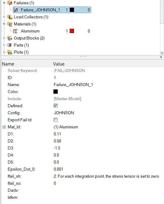
Now we can check the animation by run the simulation with default properties by following:

Analysis---->Radioss

Now we have to give location to export the input file:

Options helps to choose number of cores to solve this problem, here we have chosen 4 number of cores by (-nt 4).

Then click on Radioss, and new window will get pop-up. A simulation will start to show result,

After run the simulation on model, solver has generated different files such as engine listing file, animation, time history and then restart file.

Now, in order to check the energy error and mass error. We have to open the output file in notepad.

Once output file is opened, we can see the results.

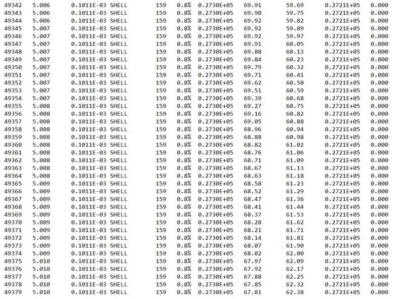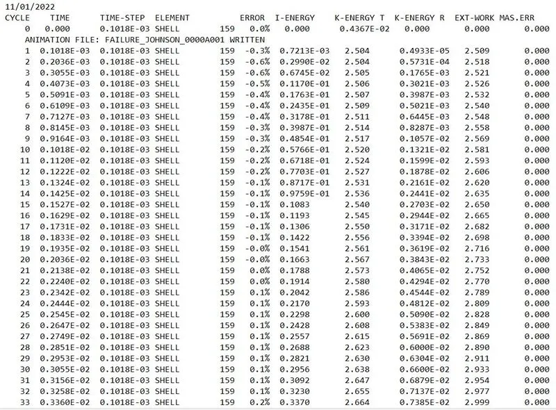
At the end of simulation, we have found maximum energy error is having value of 0.8% and maximum mass error is having value of 0.

If the energy error lies in between range of value -15 to 5%, then results will be acceptable. Also, mass error in between ranges of 0 to 2% are acceptable. If energy error is below the range, then results could be acceptable. Here we have 0.8% energy error, which is acceptable. Closer to 0%. And a mass error is coming closer to zero, which is also acceptable.

Now we have to switch from Hypermesh mode to Hyperview mode. Then we have to select the appropriated (.h3D) file. And then we have to click on Apply to view the results. Once model is opened, it will look like as shown in picture below.

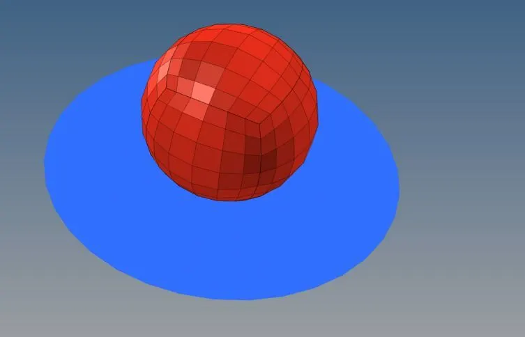
By using different animation controls, we can check and animate the results as shown in picture below.

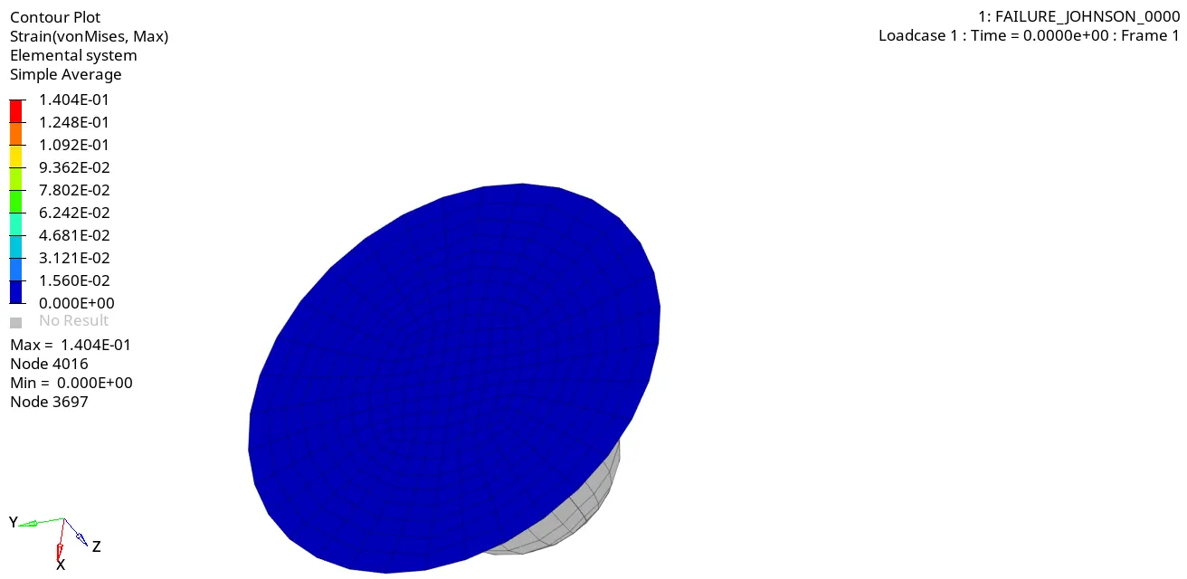
Contour plot for Von Mises stress

Maximum stress reached upto 275 MPa over the period of time.

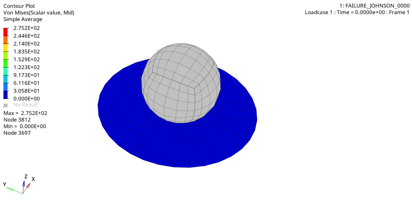
Now we have to switch from HyperView mode to HyperGraph 2D mode.

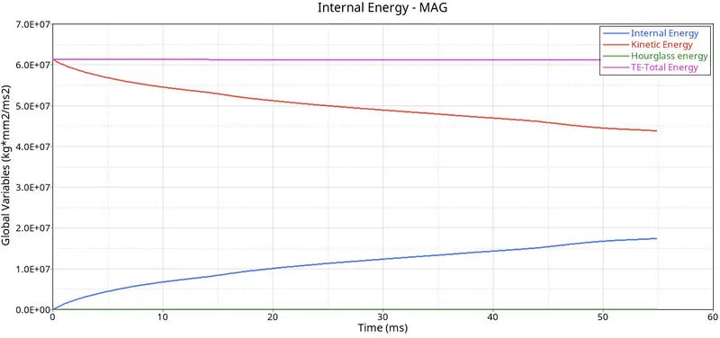
As we can see, from below graph that kinetic energy is decreasing from starting time to termination time. Because a displacement rate is reduced over a period of time. So, kinetic energy is reducing respectively.

As we know internal energy, there is no heat transfer in the system. So we only have to consider work done for calculating the internal energy. Work done is the product of force and displacement. Since a displacement is increasing over a period of time, work done will also increasing. As a result of which internal energy will also increase.

As we know total energy is the combination of internal, kinetic energy which has been plotted below.

In this case we used QEPH Ishell element formulation, so that’s the reason no hourglass deformation happened in the model. Once all parameters are filled, we have a required graph as shown in picture below.

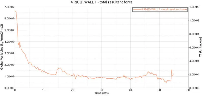
Now we have to plot the total resultant force graph. Once all parameters are filled, we have a required graph as shown in picture below.

Initially plate has more stiffness, so it took more force to press on it. With the increasing passage of time, stiffness of plate decreases as resultant force also decreases.

CASE 2: To run the model by changing given failure parameters

For this case we have to import the required file i.e. FAILURE_JOHNSON_0000.

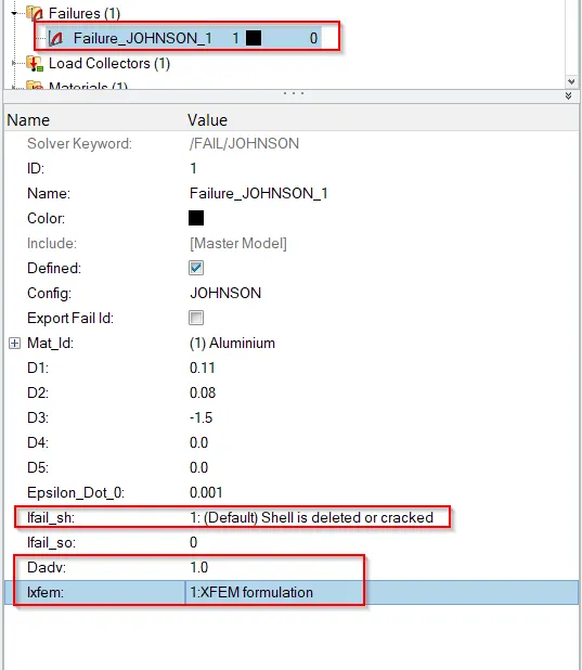
In this case we have to edit some parameters, such as Ifail_sh=1, Dadv=1, and Ixfem=1.

Ifail_sh stands for Shell failure flag, which enable Shell is deleted or cracked for one integration point or layer.

Dadv is the Criterion for the crack advancement (Only active if with Ixfem =1)

And Ixfem is failure type, in which element is either deleted or cracked.

Once required parameters are assigned, then we will save our model with name i.e. Law2_epsmax_failure. And failure card will look like as shown in picture below.

Now in order to run simulation, we have to follow same procedure as explained earlier for Case 1.

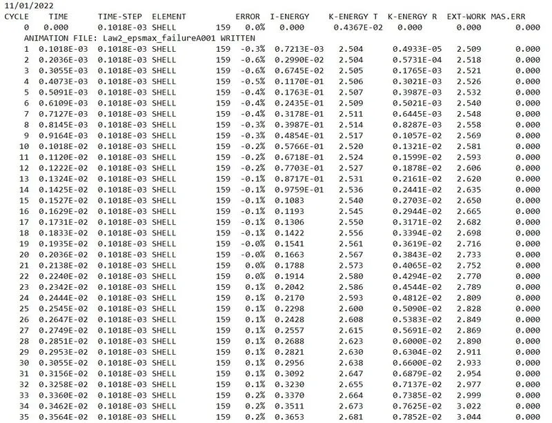
Once simulation is done, solve will generate different files. Now, in order to check the energy error and mass error. We have to open the output file in notepad.

Once output file is opened, we can see the results.

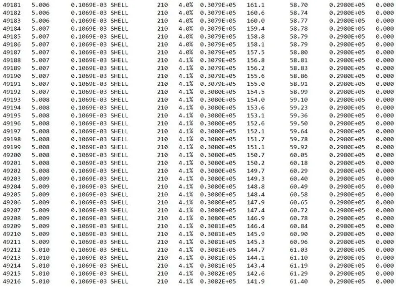So, maximum energy error is 4.1% and mass error is 0. And both are in acceptable range.

Now we have to switch from Hypermesh mode to Hyperview mode. Then we have to select the appropriated (.h3D) file. And then we have to click on Apply to view the results.

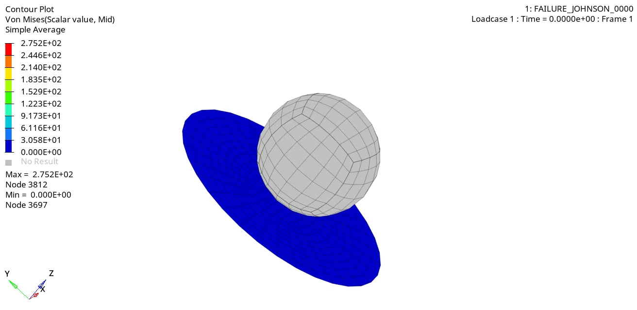
By using different animation controls, we can check and animate the results as shown in picture below.

Contour plot for Von Mises stress

Maximum stress reached upto 275 MPa over the period of time.

Now we have to switch from HyperView mode to HyperGraph 2D mode.

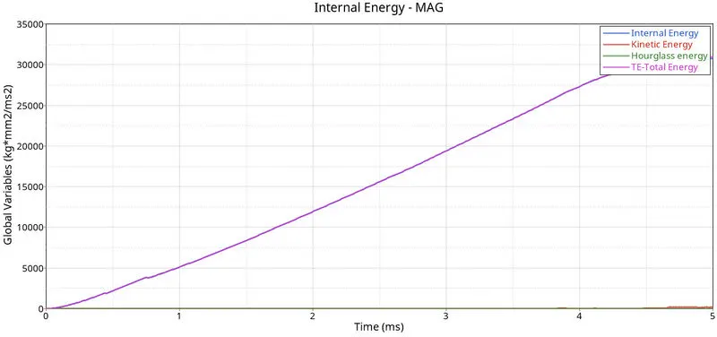
In this case, only internal energy has been developed over the period of time.

As we know total energy is the combination of internal, kinetic energy. In this case total energy is equal to internal energy, which has been plotted below.

Now we have to plot the total resultant force graph. Once all parameters are filled, we have a required graph as shown in picture below.

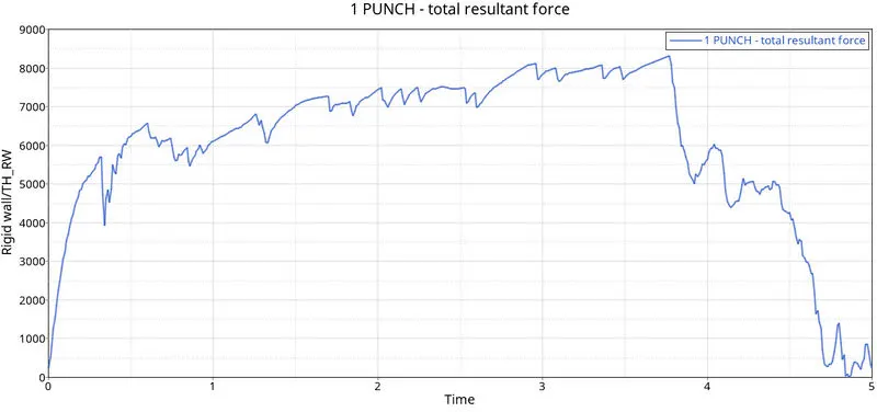
At time t=0, rigid wall force is zero. and there was no contact between ball and rupture plate. So plate element was not exerting any force to rigid ball.

At time when rigid ball hit the plate, then rigid force starts increasing. And curve pattern we will get is in zig-zag pattern. The reason behind zig-zag pattern is noise and vibration associated with sudden impact.

At ultimate strength point, rupture plate elements start breaking. And rigid ball loose its contact with plate. Hence, rigid wall force starts decreasing.

Some elements, are still in contact with rigid ball, so curve plot shows us zig zag pattern at lower rigid force.

CASE 3: To run the model by deleting failure parameters.

For this case we have to import the required file i.e. FAILURE_JOHNSON_0000.

In this case we have to delete the failure card in the model browser.Once required parameters are done, then we will save our model with name i.e. Law2_epsmax_nofail. And model browser will look like as shown in picture below.

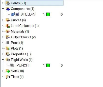
Now in order to run simulation, we have to follow same procedure as explained earlier for Case 1.

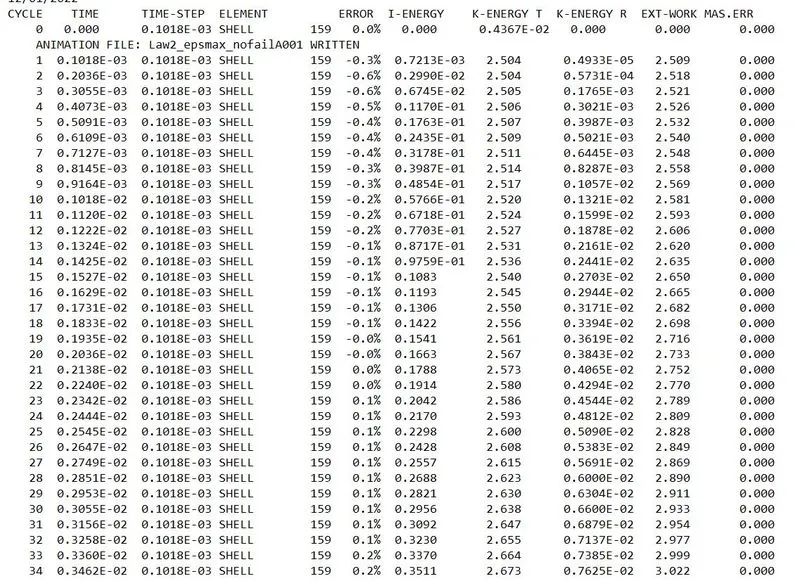
Once simulation is done, solve will generate different files. Now, in order to check the energy error and mass error. We have to open the output file in notepad.

Once output file is opened, we can see the results.

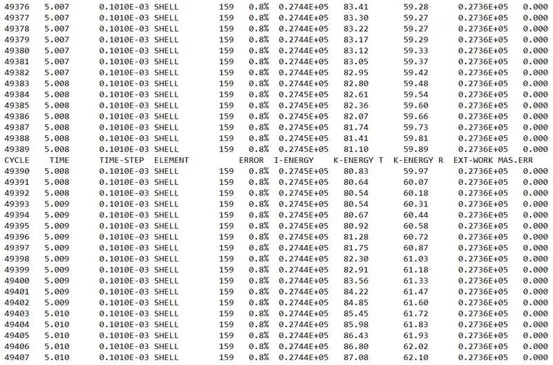So, maximum energy error is 0.8% and mass error is 0. And both are in acceptable range.

Now we have to switch from Hypermesh mode to Hyperview mode. Then we have to select the appropriated (.h3D) file. And then we have to click on Apply to view the results.

By using different animation controls, we can check and animate the results as shown in picture below.

Contour plot for Von Mises stress

Maximum stress reached upto 270 MPa over the period of time. Now it seems to generate less stress compared to case 1 and case 2. When element reaches to 15% of total strain, it deletes the element.

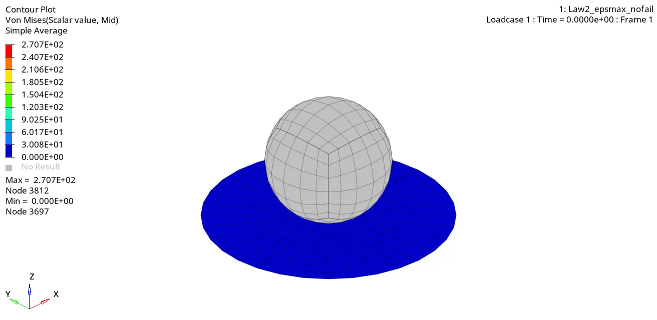
Now we have to switch from HyperView mode to HyperGraph 2D mode.

In this case, only internal energy has been developed over the period of time and no kinetic energy.

As we know total energy is the combination of internal, kinetic energy. In this case total energy is equal to internal energy, which has been plotted below.

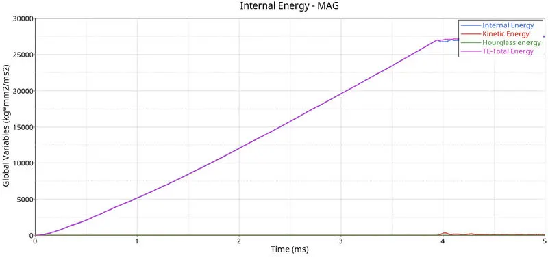
Now we have to plot the total resultant force graph. Once all parameters are filled, we have a required graph as shown in picture below.

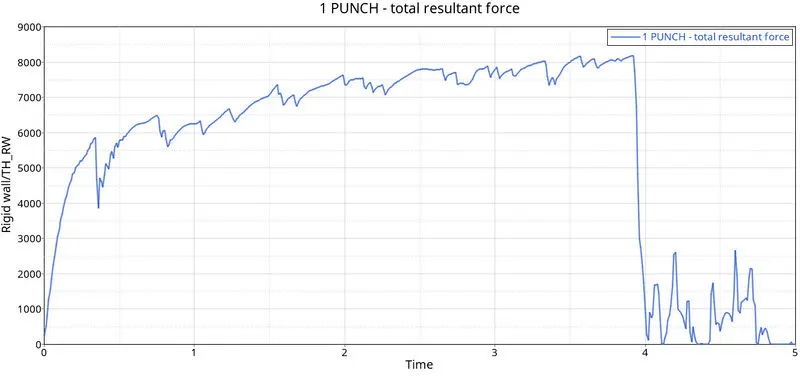
At time t=0, rigid wall force is zero. and there was no contact between ball and rupture plate. So plate element was not exerting any force to rigid ball.

At time when rigid ball hit the plate, then rigid force starts increasing. And curve pattern we will get is in zig-zag pattern. The reason behind zig-zag pattern is noise and vibration associated with sudden impact.

At ultimate strength point, rupture plate elements start breaking. And rigid ball loose its contact with plate. Hence, rigid wall force starts decreasing.

Some elements, are still in contact with rigid ball, so curve plot shows us zig zag pattern at lower rigid force.

CASE 4: To run the model by deleting the value of failure plastic strain(EPS_p_max).

For this case we have to import the required file i.e. FAILURE_JOHNSON_0000.

In this case we have to delete the value of EPS_p_max and change this value to 0 in the material card of model browser.

Once required parameters are done, then we will save our model with name i.e. Law2. And model browser will look like as shown in picture below.

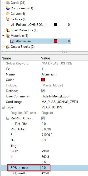
Now in order to run simulation, we have to follow same procedure as explained earlier for Case 1.

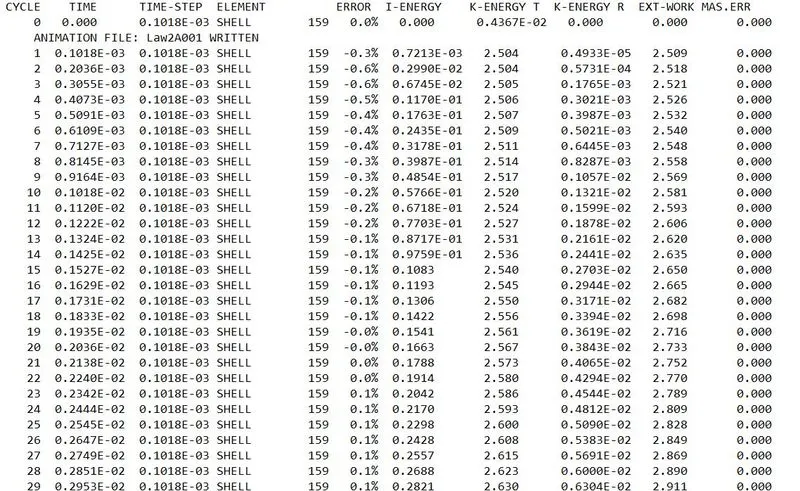
Once simulation is done, solve will generate different files. Now, in order to check the energy error and mass error. We have to open the output file in notepad.

Once output file is opened, we can see the results.

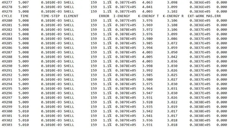So, maximum energy error is 1.1% and mass error is 0. And both are in acceptable range.

Now we have to switch from Hypermesh mode to Hyperview mode. Then we have to select the appropriated (.h3D) file. And then we have to click on Apply to view the results.

By using different animation controls, we can check and animate the results as shown in picture below.

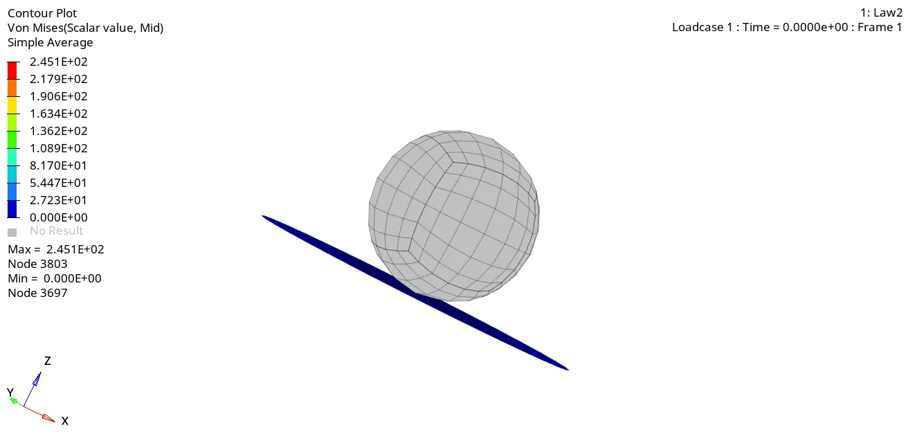
Contour plot for Von Mises stress

Maximum stress reached upto 245 MPa over the period of time. Now it seems to generate less stress compared to case 1,2 and case 3. When element reaches to 15% of total strain, it deletes the element.

Now we have to switch from HyperView mode to HyperGraph 2D mode.

In this case, only internal energy has been developed over the period of time and no kinetic energy.

As we know total energy is the combination of internal, kinetic energy. In this case total energy is equal to internal energy, which has been plotted below.

Now we have to plot the total resultant force graph. Once all parameters are filled, we have a required graph as shown in picture below.

At time t=0, rigid wall force is zero. and there was no contact between ball and rupture plate. So plate element was not exerting any force to rigid ball.

At time when rigid ball hit the plate, then rigid force starts increasing. And curve pattern we will get is in zig-zag pattern. The reason behind zig-zag pattern is noise and vibration associated with sudden impact.

At ultimate strength point, rupture plate elements start breaking. And rigid ball loose its contact with plate. Hence, rigid wall force starts decreasing.

Some elements, are still in contact with rigid ball, so curve plot shows us zig zag pattern at lower rigid force.

CASE 5: To convert the material model to Law1 elastic with same mechanical properties.

For this case we have to import the required file i.e. FAILURE_JOHNSON_0000.

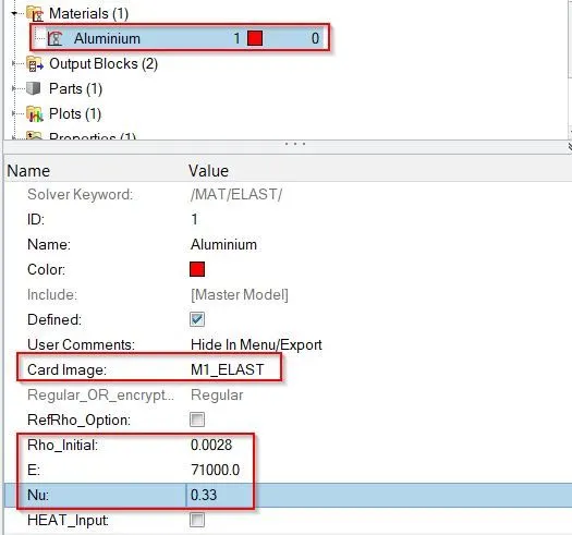
In this case we have to change the card image of material to M1_ELAST in the material card of model browser. We also have to set the value of Rho_initial, E and Nu.

Once required parameters are done, then we will save our model with name i.e. Law1. And model browser will look like as shown in picture below.

Now in order to run simulation, we have to follow same procedure as explained earlier for Case 1.

Once simulation is done, solve will generate different files. Now, in order to check the energy error and mass error. We have to open the output file in notepad.

Once output file is opened, we can see the results.

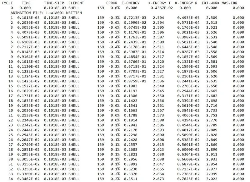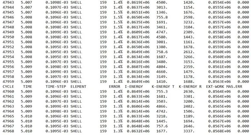So, maximum energy error is 1.3% and mass error is 0. And both are in acceptable range.

Now we have to switch from Hypermesh mode to Hyperview mode. Then we have to select the appropriated (.h3D) file. And then we have to click on Apply to view the results.

By using different animation controls, we can check and animate the results as shown in picture below.

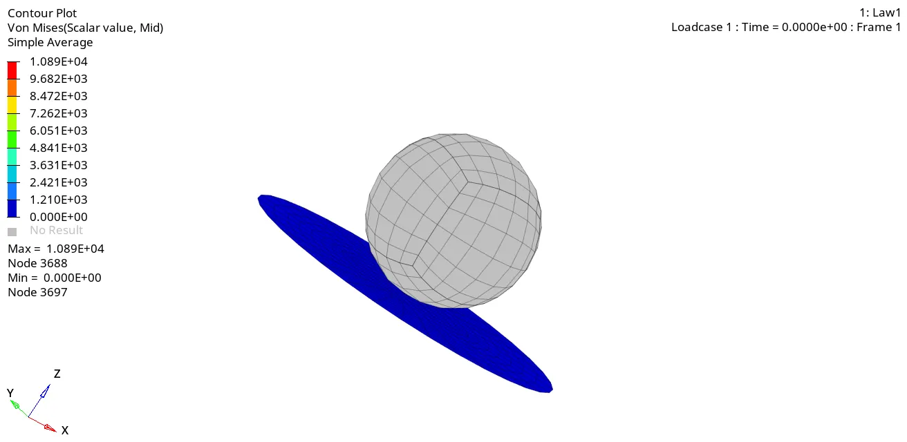
Contour plot for Von Mises stress

Maximum stress reached upto 1089 MPa over the period of time. Because of elastic material, it seems to generate more stress as compared to all previous cases.

As we can see that elements don’t crack or deleted because Eps_p_max value is set to be 0. This means an element will get fail, when it reaches to 100% of total energy. It is a ductile material, so it allows deformation without cracking or deleted.

Now we have to switch from HyperView mode to HyperGraph 2D mode.

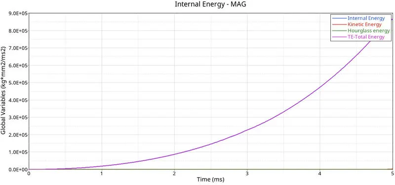
In this case, only internal energy has been developed over the period of time and no kinetic energy.

As we know total energy is the combination of internal, kinetic energy. In this case total energy is equal to internal energy, which has been plotted below.

Now we have to plot the total resultant force graph. Once all parameters are filled, we have a required graph as shown in picture below.

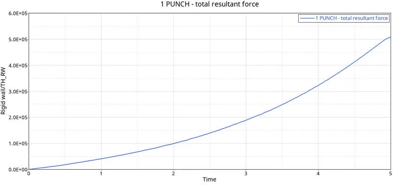
CASE 6: To run the model by using M27_PLAS_BRIT, change the shell properties to recommended shell properties and Johnson cook parameters but different value for EPS based failure.

For this case we have to import the required file i.e. LAW27_0000. It is an isotropic elastoplastic Johnsoncook material model with an orthotropic brittle failure model.

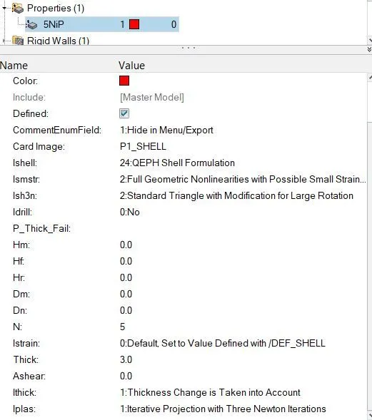
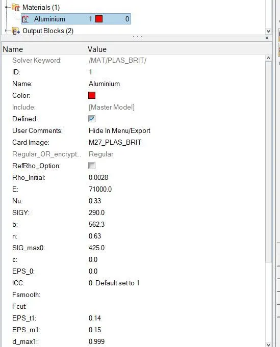
Change the material card into recommended shell properties as shown in picture below.

Once required parameters are done, then we will save our model with name i.e. Law27. And model browser will look like as shown in picture below.

BEFORE	AFTER

Now in order to run simulation, we have to follow same procedure as explained earlier for Case 1.

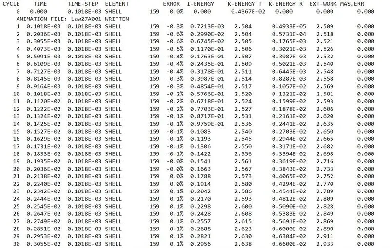
Once simulation is done, solve will generate different files. Now, in order to check the energy error and mass error. We have to open the output file in notepad.

Once output file is opened, we can see the results.

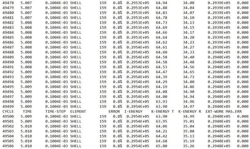So, maximum energy error is 0.8% and mass error is 0. And both are in acceptable range.

Now we have to switch from Hypermesh mode to Hyperview mode. Then we have to select the appropriated (.h3D) file. And then we have to click on Apply to view the results.

By using different animation controls, we can check and animate the results as shown in picture below.

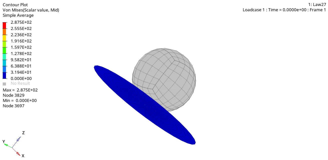
Contour plot for Von Mises stress

Maximum stress reached upto 287 MPa over the period of time. Now it seems to generate more stress compared to case 1,2,3 and case 4.

Now we have to switch from HyperView mode to HyperGraph 2D mode.

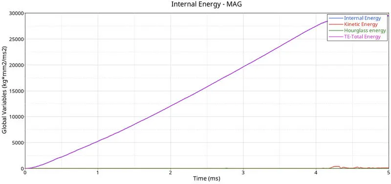
In this case, only internal energy has been developed over the period of time and no kinetic energy.

As we know total energy is the combination of internal, kinetic energy. In this case total energy is equal to internal energy, which has been plotted below.

Now we have to plot the total resultant force graph. Once all parameters are filled, we have a required graph as shown in picture below.

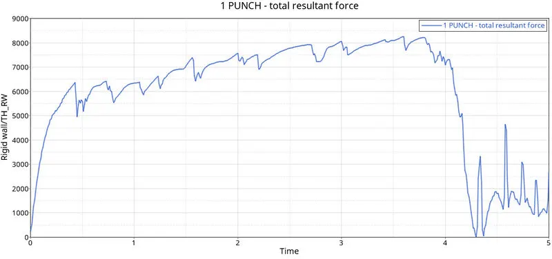
At time t=0, rigid wall force is zero. and there was no contact between ball and rupture plate. So plate element was not exerting any force to rigid ball.

At time when rigid ball hit the plate, then rigid force starts increasing. And curve pattern we will get is in zig-zag pattern. The reason behind zig-zag pattern is noise and vibration associated with sudden impact.

At ultimate strength point, rupture plate elements start breaking. And rigid ball loose its contact with plate. Hence, rigid wall force starts decreasing.

Some elements, are still in contact with rigid ball, so curve plot shows us zig zag pattern at lower rigid force.

CASE 7: To run the model by using M36_PLAS_TAB material.

In this case we have to import the required file i.e. LAW27_0000. It is an isentropic elasto-plastic material using user defined functions for the work hardening portion of the stress-strain curve for a different strain.

We have to define the stress-strain curve for this material as shown in picture below.

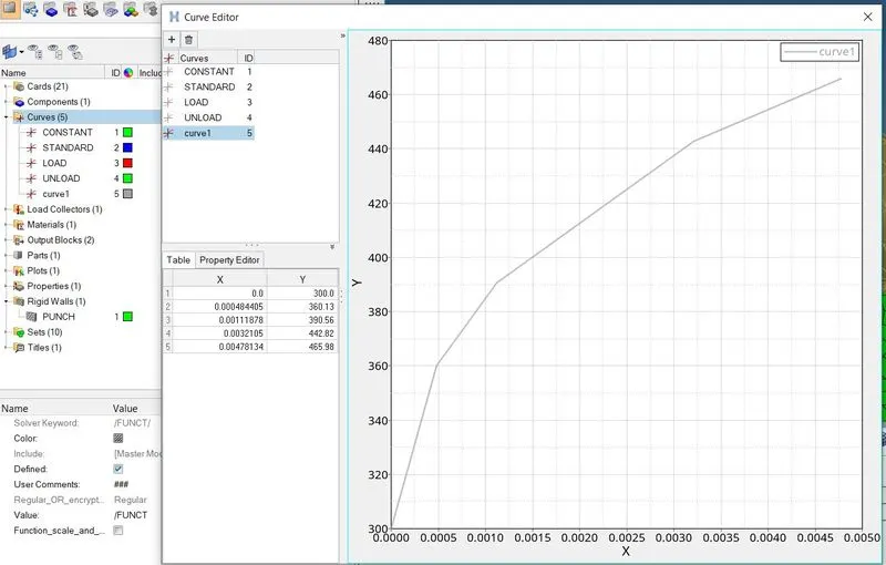
Now we have to assign newly created curve to function id as shown in picture below.

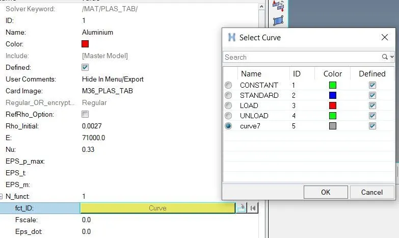
Once required parameters are done, then we will save our model with name i.e. Law36.

Now in order to run simulation, we have to follow same procedure as explained earlier for Case 1.

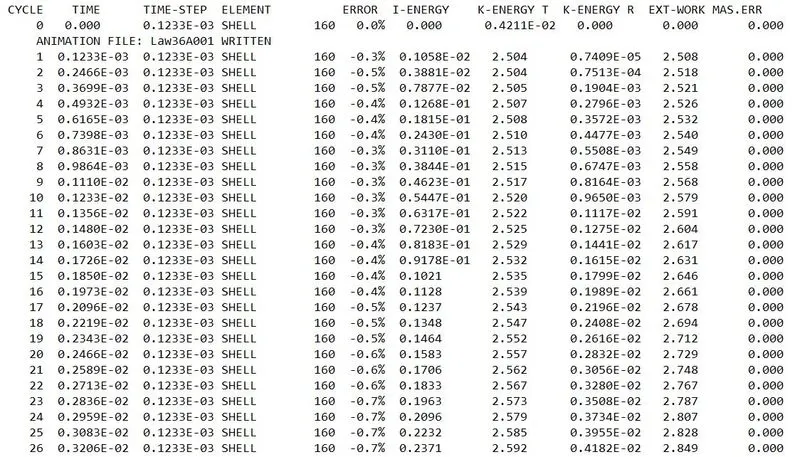
Once simulation is done, solve will generate different files. Now, in order to check the energy error and mass error. We have to open the output file in notepad.

Once output file is opened, we can see the results.

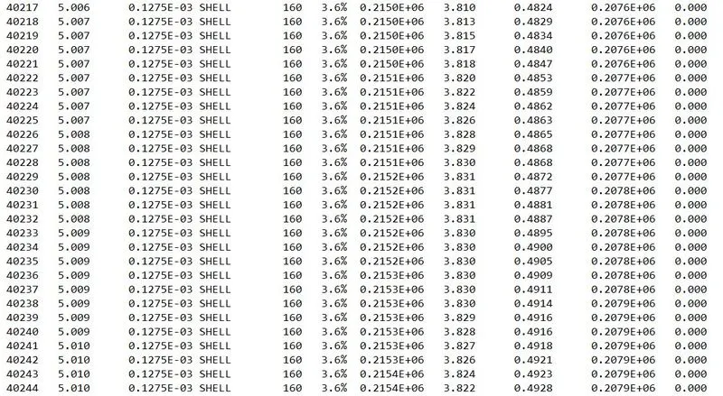So, maximum energy error is 3.6% and mass error is 0. And both are in acceptable range.

Now we have to switch from Hypermesh mode to Hyperview mode. Then we have to select the appropriated (.h3D) file. And then we have to click on Apply to view the results.

By using different animation controls, we can check and animate the results as shown in picture below.

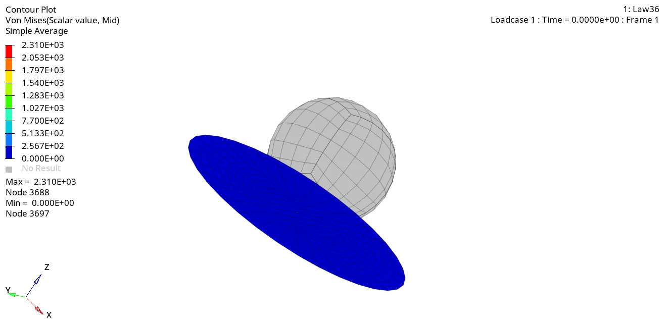
Contour plot for Von Mises stress

Maximum stress reached upto 2310 MPa over the period of time. Now it seems to generate more stress compared to above all cases.

Now we have to switch from HyperView mode to HyperGraph 2D mode.

In this case, only internal energy has been developed over the period of time and no kinetic energy.

As we know total energy is the combination of internal, kinetic energy. In this case total energy is equal to internal energy, which has been plotted below.

Now we have to plot the total resultant force graph. Once all parameters are filled, we have a required graph as shown in picture below.

At time t=0, rigid wall force is zero. and there was no contact between ball and rupture plate. So plate element was not exerting any force to rigid ball.

At time when rigid ball hit the plate, then rigid force starts increasing. And curve pattern we will get is in zig-zag pattern. The reason behind zig-zag pattern is noise and vibration associated with sudden impact.

At ultimate strength point, rupture plate elements start breaking. And rigid ball loose its contact with plate. Hence, rigid wall force starts decreasing.

Some elements, are still in contact with rigid ball, so curve plot shows us zig zag pattern at lower rigid force.

CONCLUSIONS

1. Selecting a correct material helps to get correct results in simulation.
2. RADIOSS works on wide variety of material such as concreate, foam, rubber and composites etc.