Assignment 4-RADIOSS Material Laws Challenge

AIM:

To run crash analysis on the given model by applying different materials laws available in Radioss and post-process the results

Objective:

To carry out simulations of the given starter files and compare the results. There shall be 7 cases (according to given parameters) and they are to be compared

primarily via animations and plots. The files to be worked on are the FAILURE_JOHNSON_0000.rad file and the LAW27_0000.rad file. The cases are as

follows:

1. Law 2 (file: FAILURE_JOHNSON_0000.rad) - base simulation.
2. Law 2 (file: FAILURE_JOHNSON_0000.rad) with Ifail_sh = 1, Dadv = 1, and Ixfem = 1.
3. Law 2 (file: starter file for case 2) with fail/JOHNSON card deleted.
4. Law 2 (file: starter file for case 3) with EPS_p_max value deleted
5. Law 1 (file: FAILURE_JOHNSON_0000.rad) with fail/JOHNSON card deleted and values for density, E, nu assigned
6. Law 27 (file: LAW27_0000.rad) with recommended shell properties
7. Law 36 (file: LAW27_0000.rad) with recommended shell properties and given reference curve.

Law1-Isotropic Elasticity

• Keyword in radioss like /MAT/Elast defines an isotropic, linear elastic material using hooks law. This law represents a linear relationship between stress and strain. its use in the truss, beam(type 3 only) shell, and solid elements.

• This law is useful for material attached to a rigid body.
• This law is used for a completely elastic material. Here material stiffness can be defined by two values, young's modulus, and poission ratios
• The formula used for young modulus calculation is G=E/(2(1+V))

Isotropic Elasto-plastic

• This law represents an isotropic elastoplastic material using the johnson-cook material model.
• This model expresses material stress is a function of strain, strain rate, and temperature.
• A built-in failure criterion based on maximum plastic strain is available.

Law36-Elastic-Plastic piecewise material

• This law model an isotropic Elastoplastic material.
• It is used in user-defined functions for the work hardening portion of the stress-strain curve ( For ex. Plastic strain vs stress).
• Its uses are for brick and shell elements.
• The elastic portion of the material stress-strain curve is defined by young modulus and poission ratio and density. Material plasticity curve can be given for the up an arbitrary number of strain rates.
• Linear interpolation of the stress-strain curve. 1.For a given strain rate 2.For a given plastic strain.
• In order to avoid poor curve interpolation during the strain calculation, a dummy curve defined for a high strain rate value can be added in the model,
• Typically the highest strain rate curve is repeated.
• The curves have to be defined such as they don't intersect themselves in the strain range being used otherwise the calculation may fail.
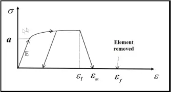
• There are some case points for the failure of elements

Viscous material-

There are two types of viscous material we study-

1. Law42-Hyper-Elastic(MAT/ODGEN or MAT/LAW42)-Odgen, Moony Rivlin

• This is of Visco Hyperelastic behavior (non-linear elastic).
• This law is generally used to model incompressible rubbers, polymers, foams, and elastomers.
• This law can be used for both shell and solid elements.
• But mainly used for polymers and elastomers.

PROCEDURE:

Case 1:

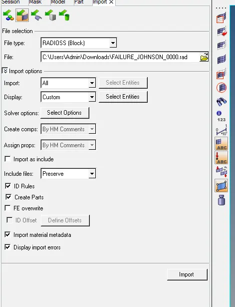
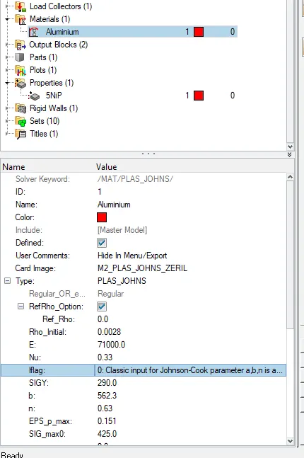
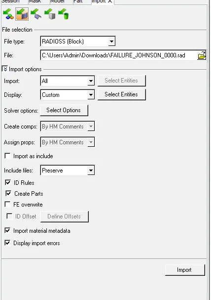
• Open Hyper mesh, go to >> import >> solver deck option >> browse File > Import. The “FAILURE_JOHNSON_0000.rad” file is selected and “imported” as shown below.

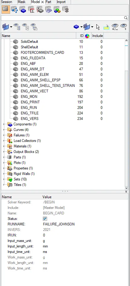
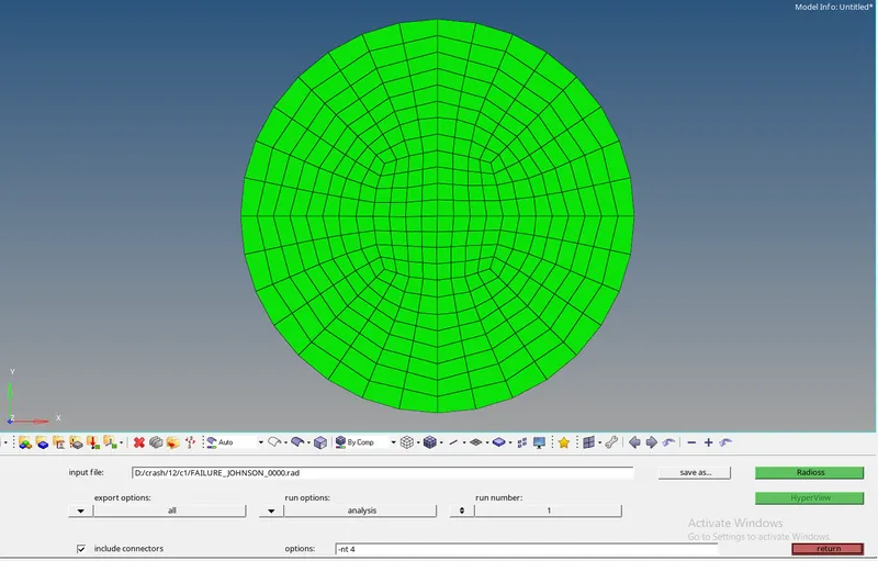
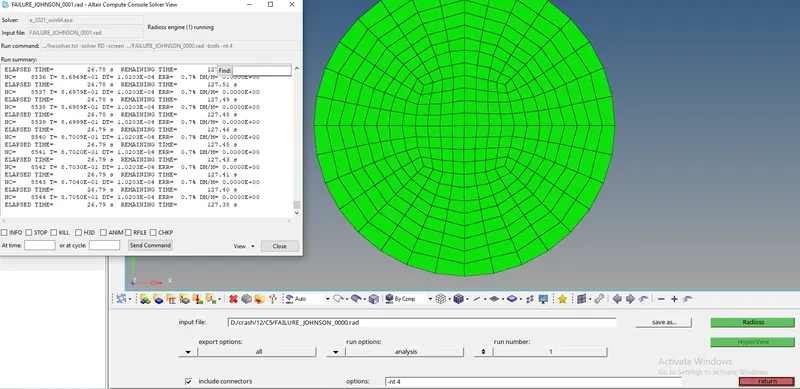
• To run the simulation, Go to Analysis >> Radioss. We need to save the output files in a new folder so that we can access them easily. The file is saved as "Law2_epsmax_failure_0000.rad". After saving, tick the 'include connectors' box and type in '-nt 4' in the options text box as shown below, before clicking 'Radioss'

• It is recommended to be written as "-nt 4" as shown in the image below. This means assigning the task to 4 cores in the system, to perform the simulation faster. It depends upon the process of our computer (it has a quad-core processor, then it should be taken as 4. If the system has an octa-core processor, then it is taken as 8). And "nt" means "number of threads". Then click on "Radioss", in order to run the simulation

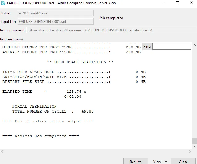
• By clicking 'Radioss', we get the solver window as shown below, which basically tells us what the RADIOSS solver is doing. After a few minutes, radios does the job and you can check all the files in the folder which you have saved as.

• The simulation is complete, now we just need to visualize it. For that, we need to switch to the Hyperview utility.
• After accessing Hyperview, we should input the simulation file. For this, use the h3d file that was generated when RADIOSS processed the starter file. It is generated in the files which are shown in the picture above. After selecting it, we can click 'apply'
• After accessing Hyperview, we are asked to input the simulation file. For this, we shall be using the h3d file that was generated when RADIOSS processed the starter file (Law2_epsmax_failure.h3d). It should be generated in the same folder. After selecting it, we can click 'apply'. Doing so generates the simulation animation
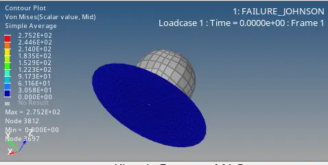
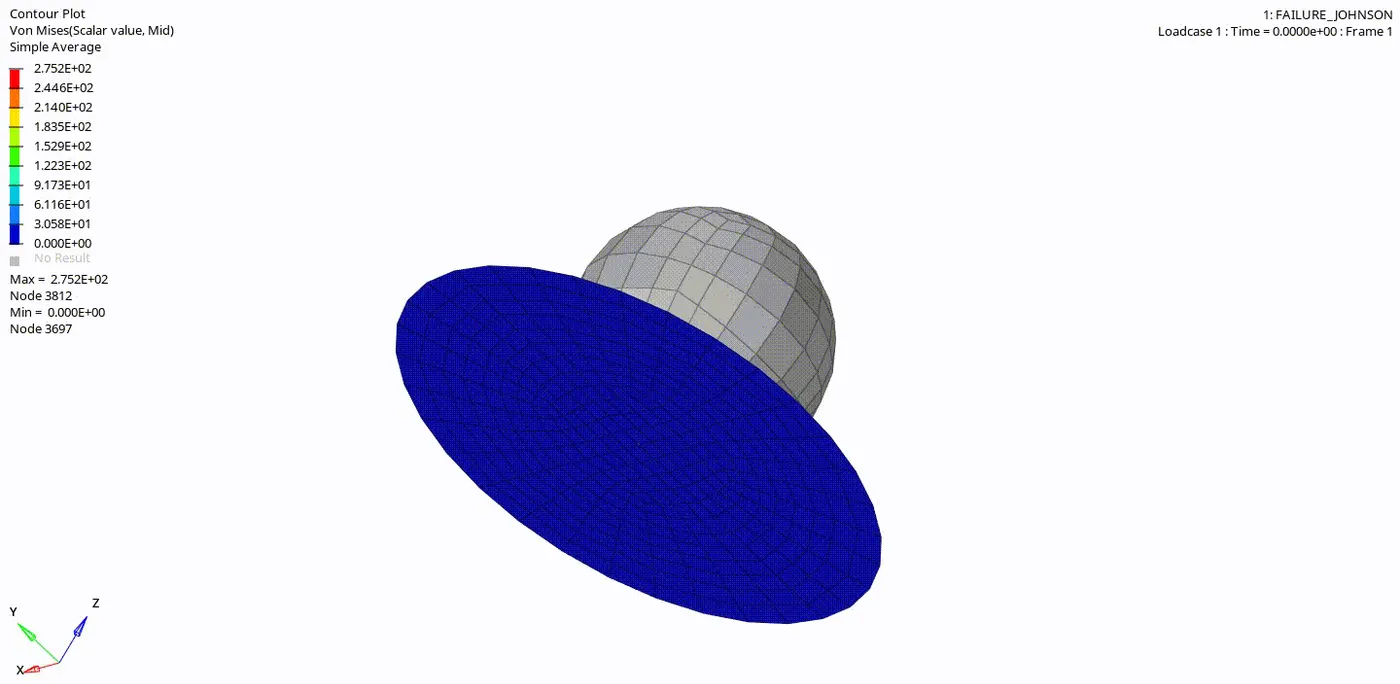
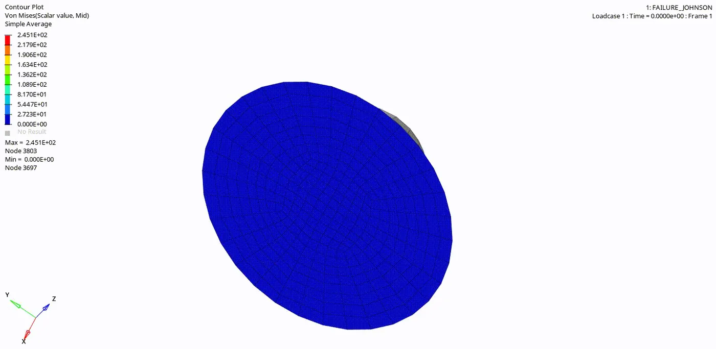
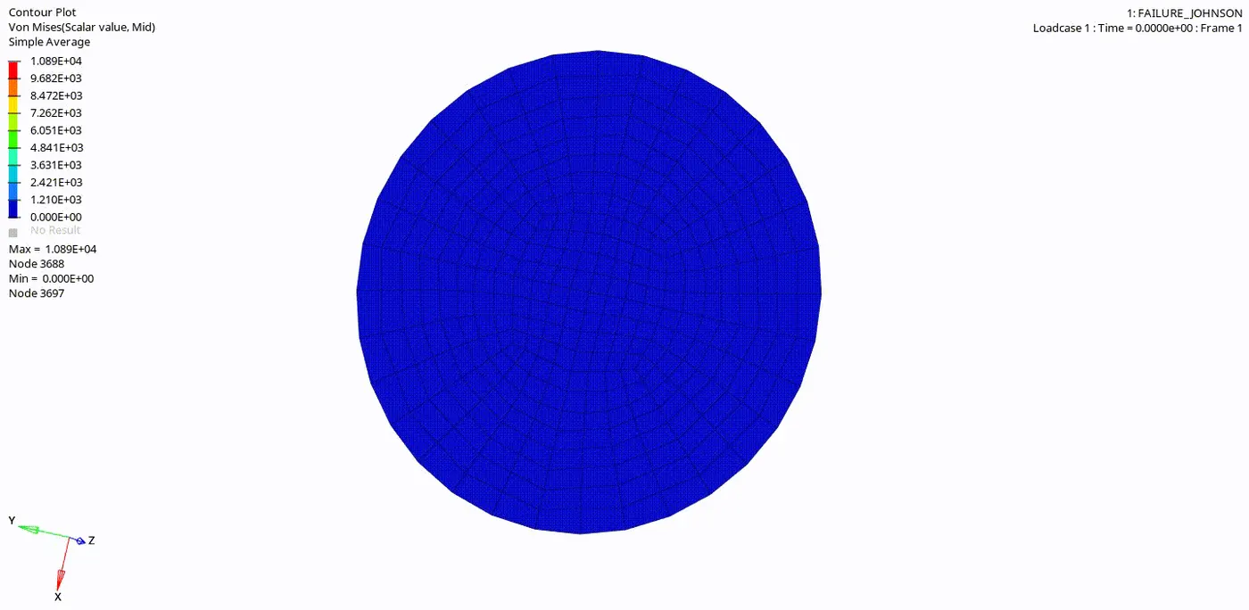
• We can change what is being represented by selecting the 'contour' option in the toolbar. In this case, we can change the result type to 'Von Mises' and change the averaging method to simple. Doing so creates the Von Mises stress contours as shown below

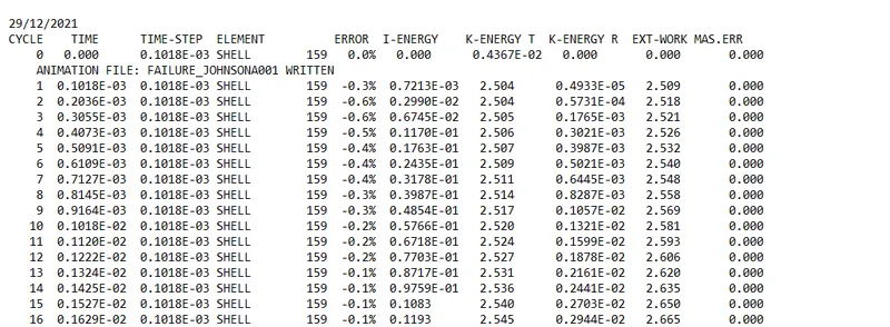
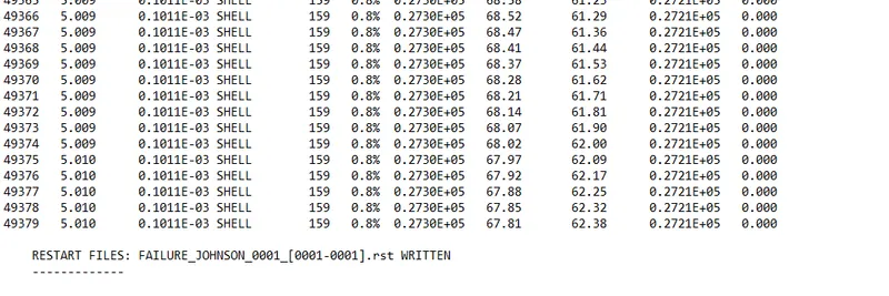
Energy error is 0.8 % Acceptable (Range is -15% to +5%)

Mass Error 0 Acceptable (Range is 0 to 2%)

• Now plot the graphs in Hypergraph 2D. We can switch to it using the same client selector option in the toolbar.
• In the Hypergraph section, we need to input a file. For this, we will be using the result file generated by the RADIOSS solver (also known as the 'T01 file'). This file is available in the same directory as the starter, engine, and animation files. The file name ends with 'T01'

Rigid Wall Force-

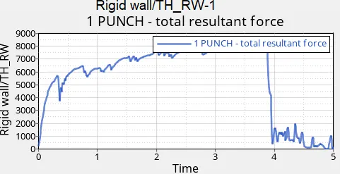
• At t=0 Rigid wall force is zero because at that time there was no contact between ball and plate. hence elements are not exerting any force to the rigid ball.
• The moment the ball hits the plate rigid force starts increasing and it will show some zig-zag behavior and that's due to noise and vibration-induced due to sudden impact.
• At the ultimate stress point elements start breaking and the ball starts losing contact with the elements that's why we can see the sudden drop in the graph.
• Since some elements were still in contact with the plate after rapture due to that we can see further zig-zag graph at a lower force.

Internal Energy-

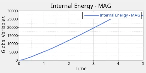
• Initially, the ball was not in contact with a circular plate so at t=0 internal energy was zero.
• And the time when the ball hits the plate there is stress generation and due to this stress, the strain will happen.
• That strain starts the deformation in the plate and due to this internal energy starts increasing.
• It will increase till the ultimate strength after those point elements start breaking and due to this element break, strain increment stopped that is why the graph is flat after the rapture point.

Kinetic Energy-

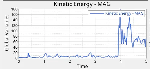
• At t=0 velocity of elements is zero because at that time there was no contact between ball and plate.
• But when the ball hits the plate then elements start moving due to deformation till plastic fracture.
• But after fracture, since elements start breaking then there is a sudden rise in the velocity of elements we can see in simulation hyper view animation.
• So due to this, there is a sudden gain in kinetic energy in elements due to rapture.

Hourglass Energy-

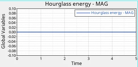
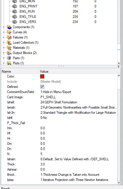
• Since we have used improved under integrated elements which are Ishell 24 (QEPH).
• So due to that, there is no hourglass is noted.

Case-2 -

Use same FAILURE JHONSON 000.rad with change in Failure criteria. (lfail_sh=1, Dadv=1, lxfem=1 )

Here in the 2nd case material Law will be the same ( LAW2) but the failure criteria will be changed.

a.lfail_sh = 1 (Default, shell is deleted or cracked)

b.Dadv = 1 (It will initiate the crack when it will reaches ultimate stress)

c.lxfem = 1 (It will delete the cracked element.)

• Give all the values in the input failure card.

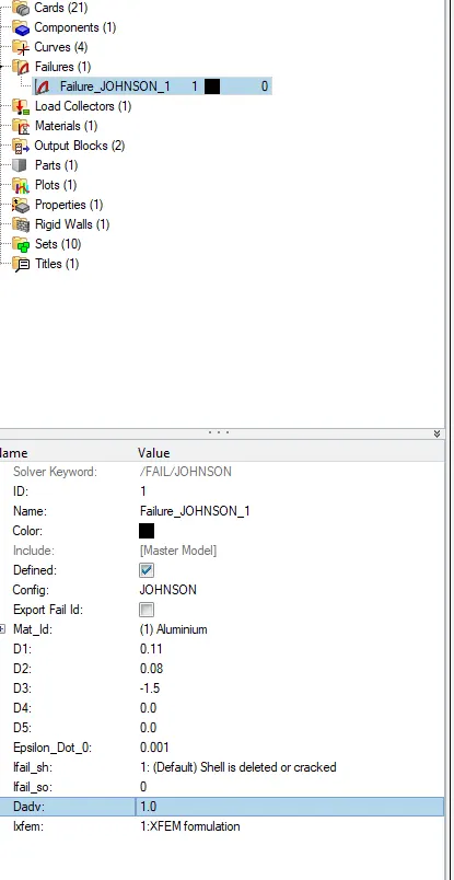
• Now run the simulation as with the edited failure card.
• After running the simulation we will see new h3d and animation will be generated

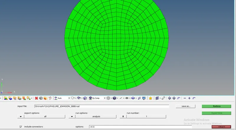
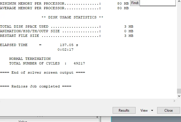
• Now open 0001.out file and check all the details.
• Here we can see all variables in the out file about energy and mass loss also.

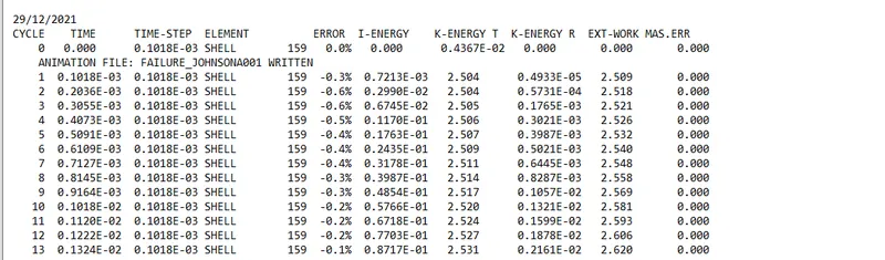
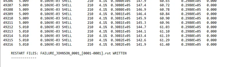
Energy error = 4.1 % Acceptable (Range is -15% to +5%)

Mass Error = 0 Acceptable (Range is 0 to 2%)

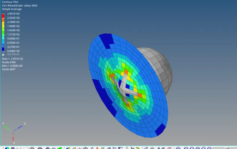
Plot the graphs using Hypergraph-2D

• After opening the hypergraph window import the T01 file in Hypergraph.

Rigid wall force Graph-

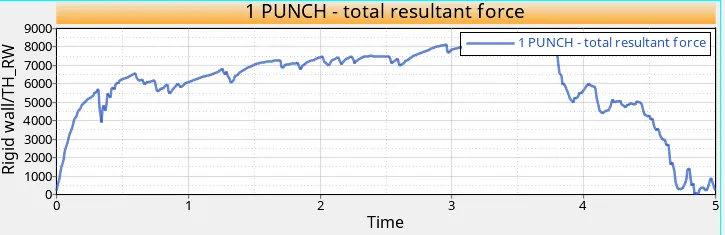
• At t=0 Rigid wall force is zero because at that time there was no contact between ball and plate.
• The moment the ball hits the plate rigid force starts increasing and it will show some zig-zag behavior and that's due to noise and vibration-induced due to sudden impact.
• At the ultimate stress, point elements start breaking and the ball starts losing contact with the elements that's why we can see the sudden drop in the graph.
• But in this case, we can see less drop in the Rigid force graph after breaking compared to case-1. Because in case-2 more elements are in contact with the ball during simulation

Internal Energy-

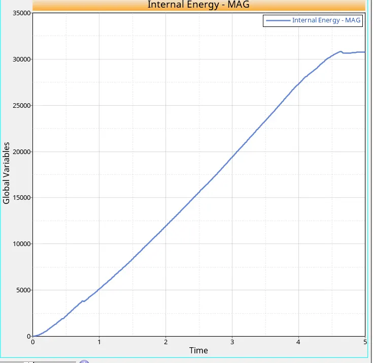
• It will increase till ultimate strength because deformation is taking place and due to deformation strain energy is generated and that energy is stored in the form of internal energy.
• After those point elements start breaking and due to this element break, strain increment stopped that is why the graph is flat after rapture point

Hourglass Energy

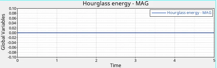
• Since we have used improved under integrated elements which are Ishell 24 (QEPH).
• So due to that, there is no hourglass is noted.

Kinetic Energy-

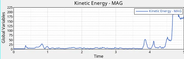
• At t=0 velocity of elements is zero because at that time there was no contact between ball and plate.
• But when the ball hits the plate then elements start moving due to deformation till plastic fracture and due to deformation strain energy is storing so that's why kinetic energy not increasing that much.
• But after fracture, since elements start breaking and moving at a faster rate then there is a sudden rise in the velocity of elements we can see in simulation hyper view animation.
• The ad then it's decreasing slightly because of losing contact.

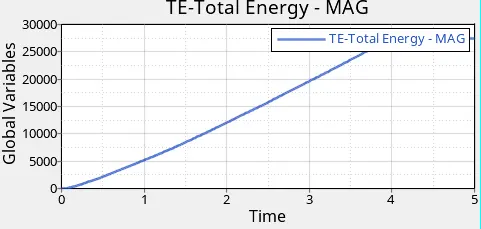
Total energy-

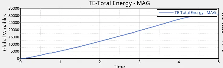
• The total energy is the sum of all types of energy present here, Kinetic+Internal+contact+hourglass.
• So it will increase as all energies combinedly increase.

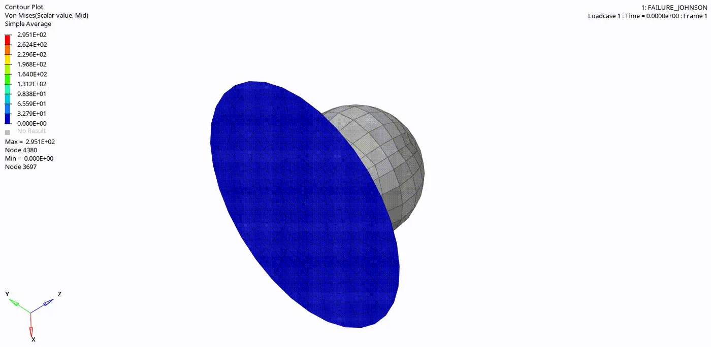
Case-3-

Delete the failure card (fail/JHONSON)

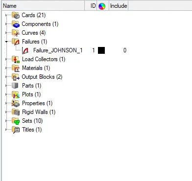
• Now run the simulation and save the radios file as different case as case-3.
• After running the simulation we will get the animation file, h3d file, and also T01 file.

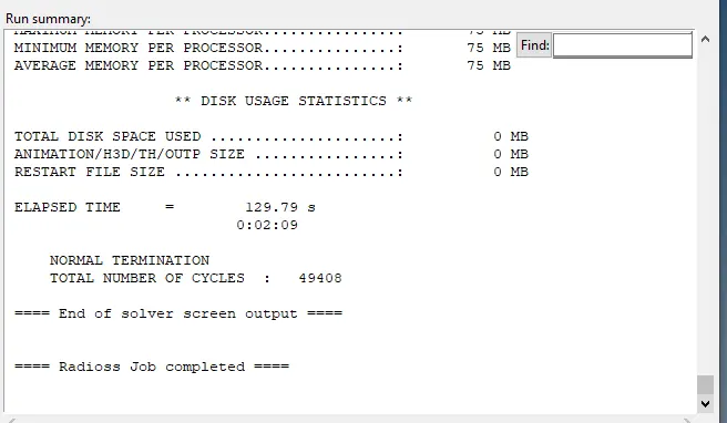
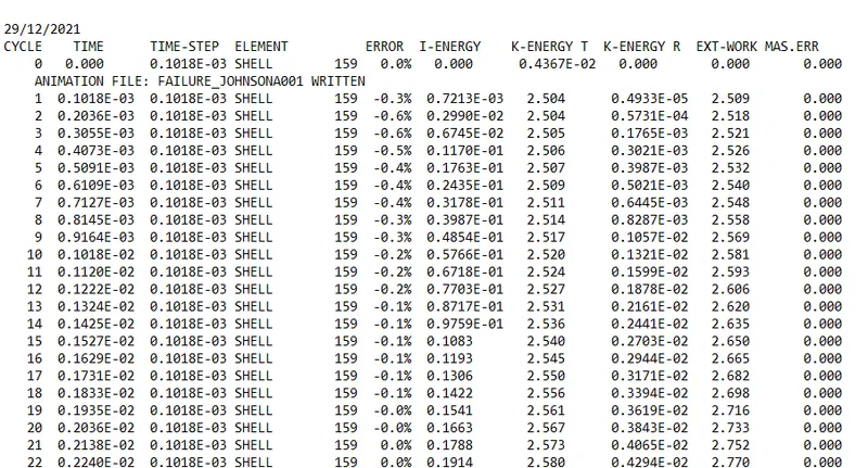
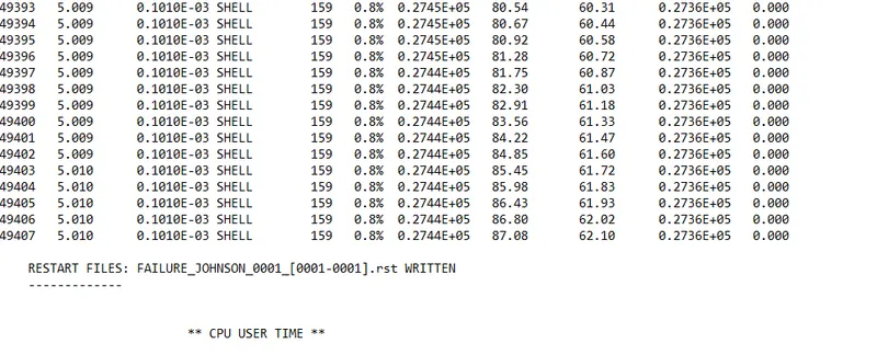
Energy error = 0.8 % Acceptable (Range is -15% to +5%)

Mass Error = 0 Acceptable (Range is 0 to 2%)

Plot the graphs using Hypergraph-2D

• After opening the hypergraph window import the T01 file in Hypergraph.

Rigid wall force Graph-

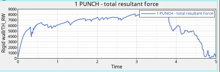
• Here rigid wall force graph variation is looking similar to case-1 because the element failure and breaking is similar to case-1.
• Most of the elements are break loose from the plate that's why after the ultimate point graph falls suddenly after that also some remaining elements exerted some force on ball that's why the graph is continued in that way as shown above.

Internal Energy-

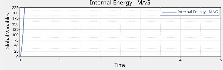
• It increases till the ultimate strength point because till that point deformation takes place.
• And due to deformation, the internal energy is recorded.
• But after the breaking point element loses the contact so that no deformation is happening that's why the graph is being constant after that point.

Kinetic Energy-

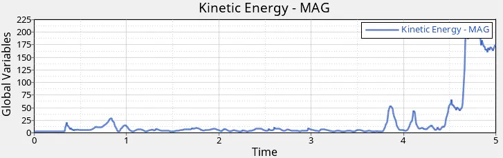
• Here in this case very less amount of kinetic energy is being noticed because while the ball is colliding with the plate most of the energy is converted into strain energy.
• But after the ultimate strain point due to elemental break sudden increase in the kinetic energy graph is noted.

Hourglass energy-

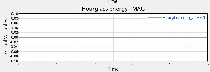
• Since we have used improved under integrated elements which are Ishell 24 (QEPH).
• So due to that, there is no hourglass is noted.

Total Energy-

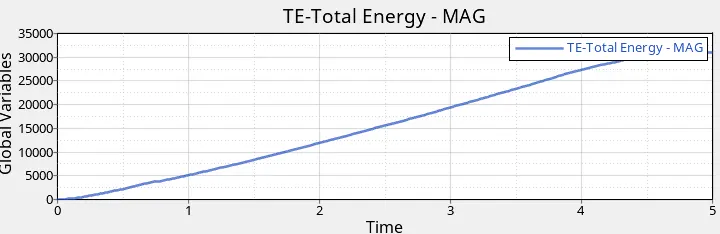
• The total energy is the sum of all types of energy present here, Kinetic+Internal+contact+hourglass.
• So it will increase as all energies combinedly increase.

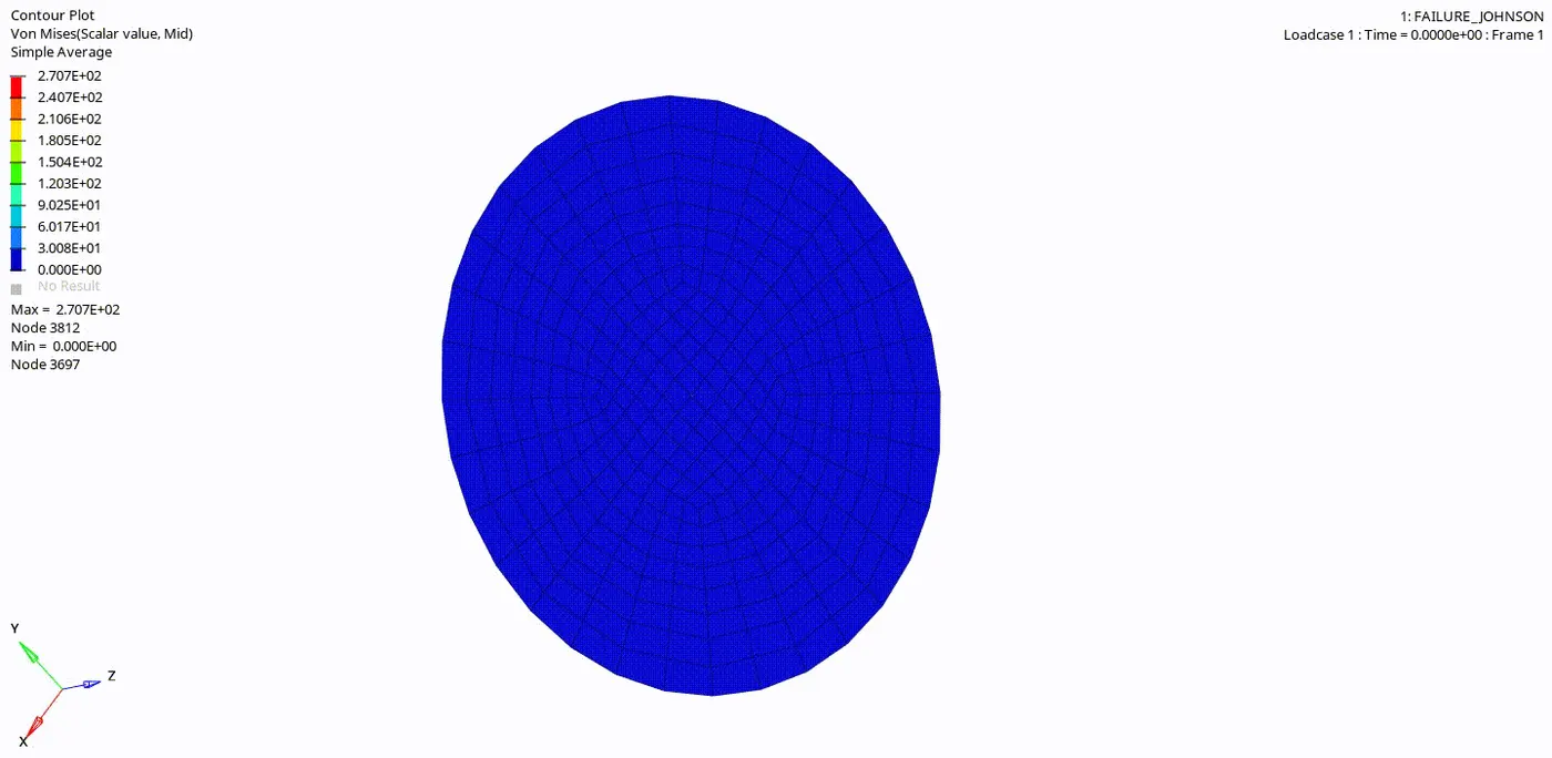
Case-4-

Delete the Epx_p_max value from material card.

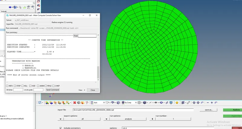
• Now run the simulation and save the radios file as different case as case-4.
• After running the simulation we will get the animation file, h3d file, and also T01 file.

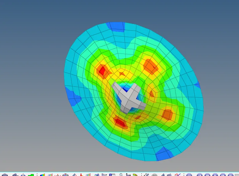
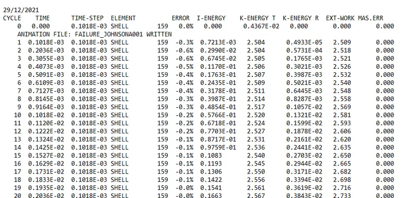
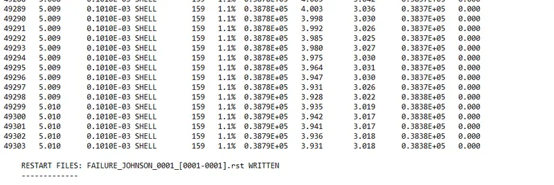
Energy error = 1.1 % Acceptable (Range is -15% to +5%)

Mass Error = 0 Acceptable (Range is 0 to 2%)

Plot the graphs using Hypergraph-2D

• After opening the hypergraph window import the T01 file in Hypergraph.

Rigid wall force Graph-

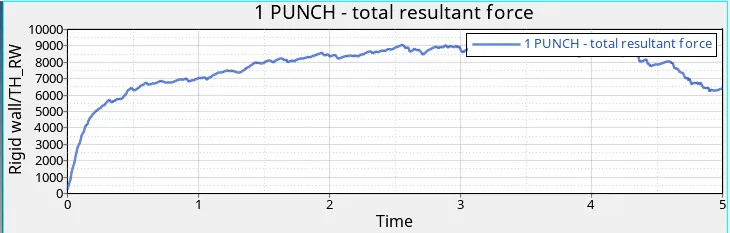
• Here, in this case, there is not such kind of sudden drop in the graph, because there is no defined value for maximum strain by the user.
• So it will continue increasing till the original maximum strain value with some zig-zag pattern due to noise.
• And after reaching the original max strain value it will break and then elements start deleting and losing contact with the rigid ball, that's why the graph is decreaing slightly after some time.

Internal Energy-

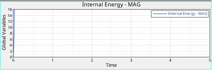
• Internal energy keeps on increasing since there is no specific value for maximum strain given by the user.
• The graph is not constant after some time like in previous cases is just because the elements in the previous case are break and fall apart, and after falling apart solver record no strain energy(because it will not deform after falling apart) that's why the graph was constant.
• But in this case, no elements are falling apart, yes some elements are breaking deleted so that solver will not record their internal energy value.

Kinetic Energy-

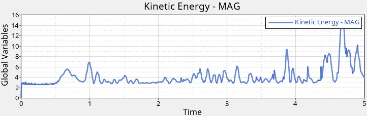
• Here initially there will be some kinetic energy present because elements are deforming at low speed, cause we have not given a specific Eps_max value.
• so it will take time to deform and to reach its original Eps_max value.
• Along with time when it starts deforming properly elements also start moving a little faster so there is a gain in kinetic energy.
• And it will follow the same zig-zag pattern till the ultimate strength of Aluminum or can say original Eps_max of Aluminum.

Hourglass Energy-

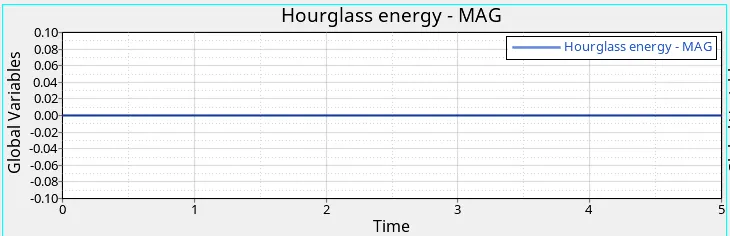
• Since we have used improved under integrated elements which are Ishell 24 (QEPH).
• So due to that, there is no hourglass is noted.

Total energy

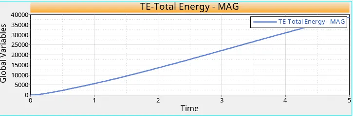
• The total energy is the sum of all types of energy present here, Kinetic+Internal+contact+hourglass.
• It will follow the same pattern as internal energy.

Case-5-

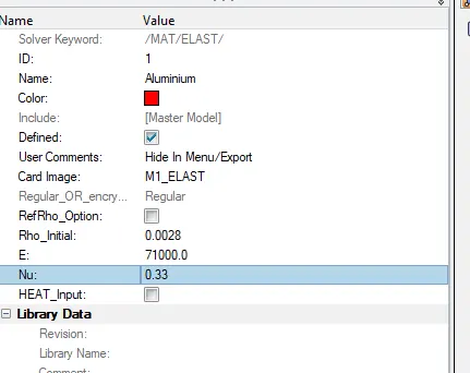
Change the material card to Law1 with the same E and rho value.

• Now run the simulation and save the radios file as different case as case-5.
• After running the simulation we will get the animation file, h3d file, and also T01 file.

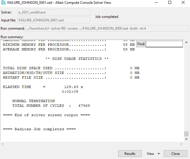
Energy error = 1.3 % Acceptable (Range is -15% to +5%)

Mass Error = 0 Acceptable (Range is 0 to 2%)

• Review the simulation using Hyperview.
• Plot the graphs using Hypergraph-2D

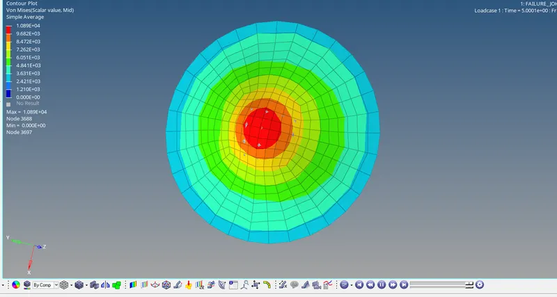
Plot the graphs using Hypergraph-2D

• Now split the window in 3Part and open hypergraph-2D in the new window.
• After opening the hypergraph window import the T01 file in Hypergraph.

Rigid wall force Graph-

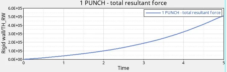
• In this case, when the ball hits the elastic plate there is gradual deformation takes place but elements will not delete since it is elastic material we had assigned.
• Since the ball collides with the elastic plate so due to this a force is exerted by elements to the ball and that force will increase gradually
• Because the element is not deleting and it will be always in contact so, as deformation is taking place in that way rigid wall force will also increase.

Internal Energy-

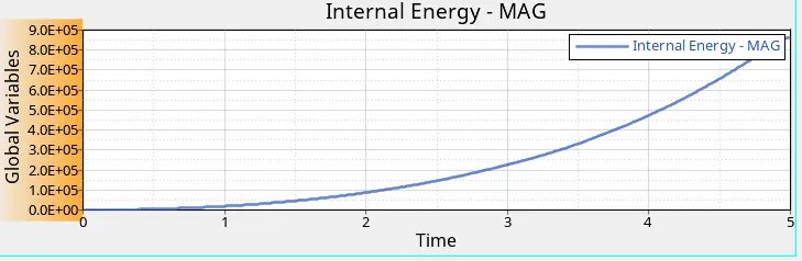
• In this case, due to gradual deformation strain energy will also increase in the same way. And that energy is internal energy stored in the plate.
• Here elements are not breaking so it will keep increasing.

Kinetic Energy-

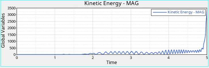
• Initially, in this case, the kinetic energy of elements is less due to small deformation.
• But with respect to time deformation is taking place so that there is a slight increment in kinetic energy we can see from the graph.
• And it will end at a higher value since deformation is keep increasing.

Hourglass energy-

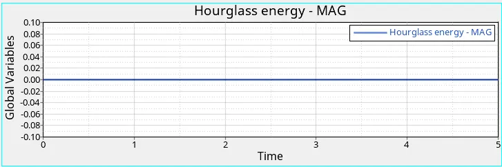
• Since we have used improved under integrated elements which are Ishell 24 (QEPH).
• So due to that, there is no hourglass is noted.

Total Energy-

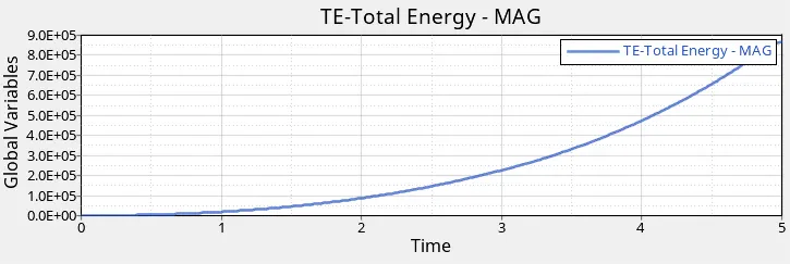
• The total energy is the sum of all types of energy present here, Kinetic+Internal+contact+hourglass.
• It will follow the same pattern as internal energy.

Case-6-

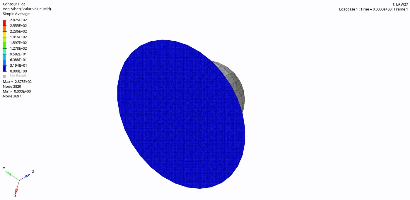
Change the material card to Law27

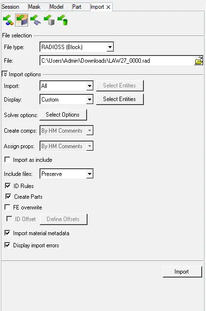
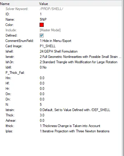
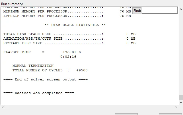
• Now run the simulation and save the radios file as different case as case-6.
• After running the simulation we will get the animation file, h3d file, and also T01 file.

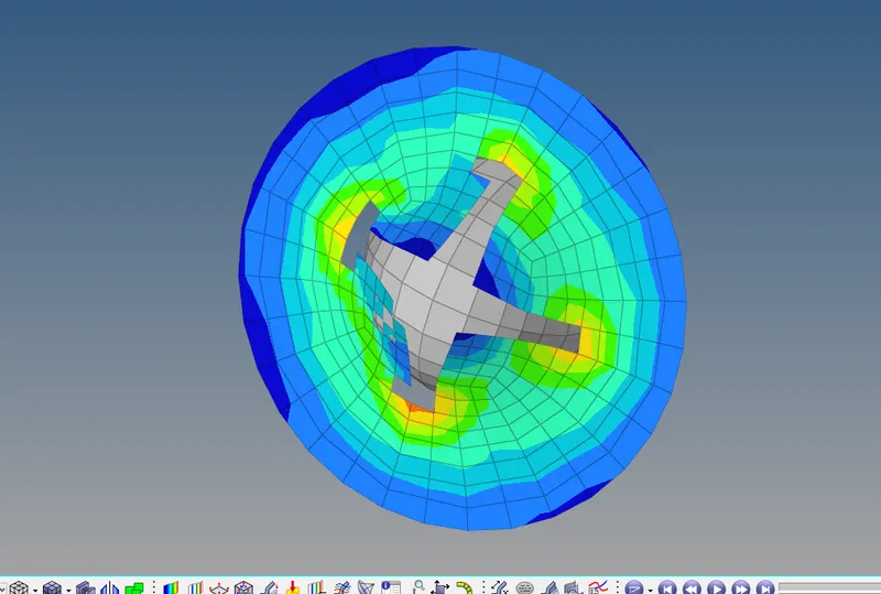
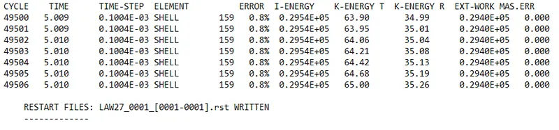
Energy error = 0.8 % Acceptable (Range is -15% to +5%)

Mass Error = 0 Acceptable (Range is 0 to 2%)

Plot the graphs using Hypergraph-2D

• After opening the hypergraph window import the T01 file in Hypergraph.

Rigid wall force Graph-

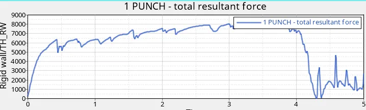
• In this also like precious cases elements will break after some time and can see a sudden drop in the graph.
• After the maximum strain point, some material is still in contact with the ball so rigid wall force act from that material as shown in the graph.

Internal Energy-

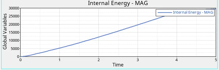
• Internal energy increase linearly and after the maximum strain point, it will get disturbed due to material failure as shown above.

Kinetic Energy-

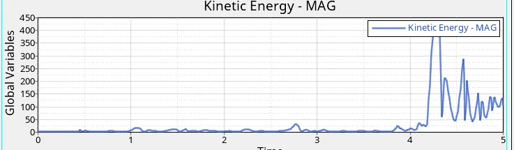
• Kinetic energy is slightly low initially and after maximum strain point because till that point, most of the energy gets absorbed as internal energy.
• After that elements are breaking and start moving away then that energy is converted into kinetic energy.

Hourglass energy-

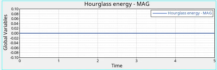
• Since we have used improved under integrated elements which are Ishell 24 (QEPH).
• So due to that, there is no hourglass is noted.

Total Energy-

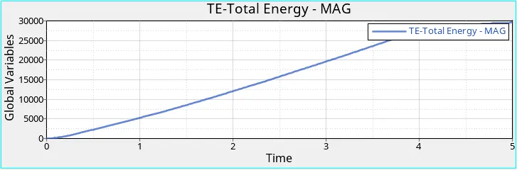
• The total energy is the sum of all types of energy present here, Kinetic+Internal+contact+hourglass.
• It will follow the same pattern as internal energy.

Case-7-

Change the material card as Law36

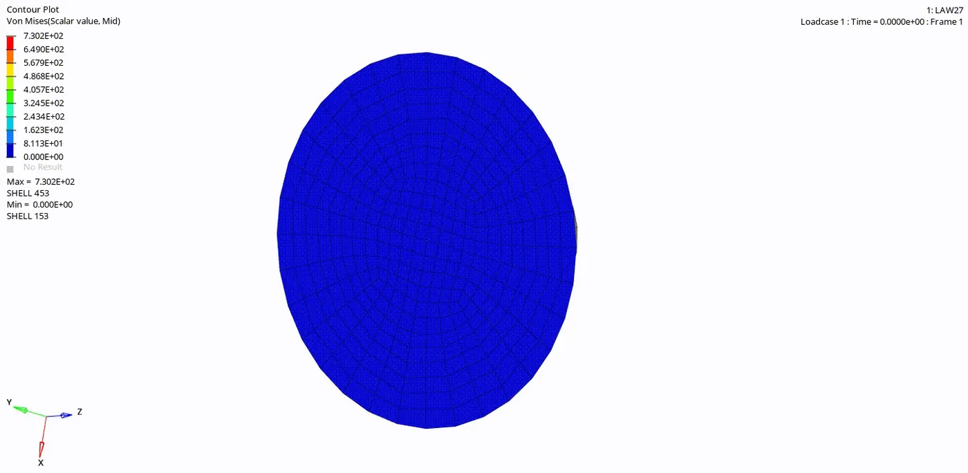
• After changing the mat. card shell parameter will also turned to default.
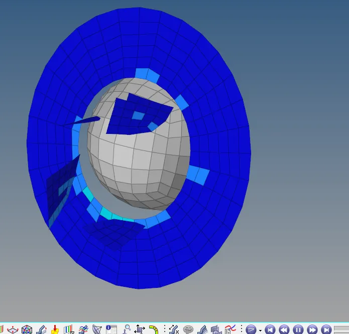
• Now assign the required shell parameter.

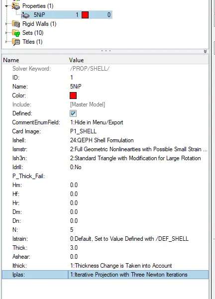
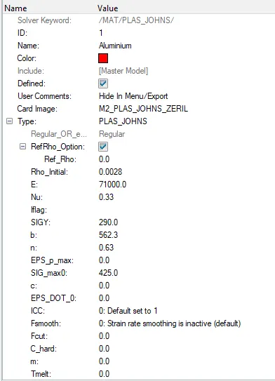
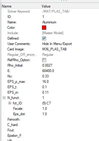
• Now go to Materials >> Aluminium and change the card to M36_PLAS_TAB (Law 36). After that, set the values for Rho_Initial, E & Nu as follows: Rho_initial = 0.0027, E = 71000.00, nu = 0.33.
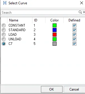
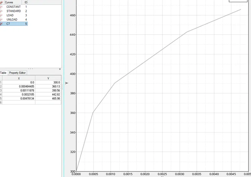
• We can then add the curve using the N_funct attribute. We can change its value to 1 and by doing so, it lets us select the reference curve. We shall select the one we just made.
• Now set all the material property values according to the mat card we have.

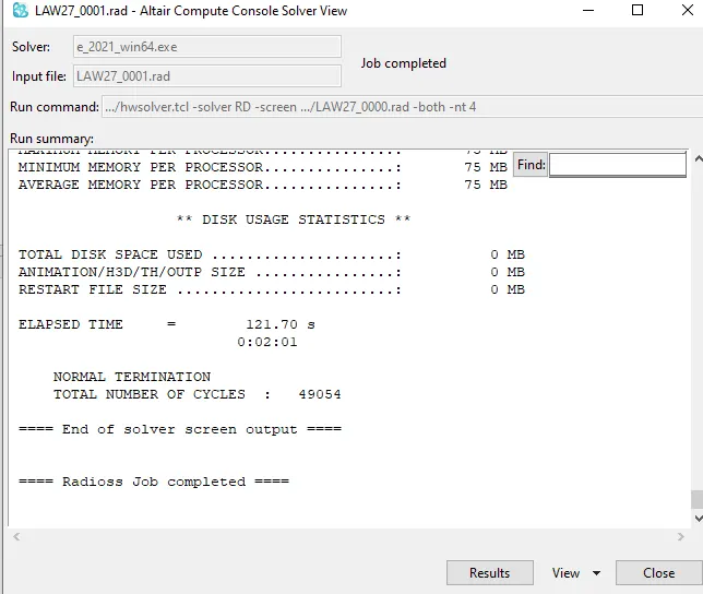
• Now run the simulation after this and check for results.
• After running the simulation we will get the animation file, h3d file, and also T01 file.

Energy error = -2.3 % Acceptable (Range is -15% to +5%)

Mass Error = 0 Acceptable (Range is 0 to 2%)

Plot the graphs using Hypergraph-2D

• After opening the hypergraph window import the T01 file in Hypergraph.

Rigid wall force Graph-

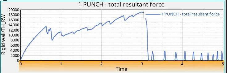
• Rigid wall force increase till the point of maximum strain value cause till that point elements are in contact with the rigid ball.
• After losing contact rigid wall force drop-down drastically cause most of the elements are break and move away.

Internal Energy-

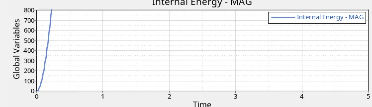
• Till plastic failure internal energy keeps increasing as it stores strain energy due to the deformation of elements.

Kinetic Energy-

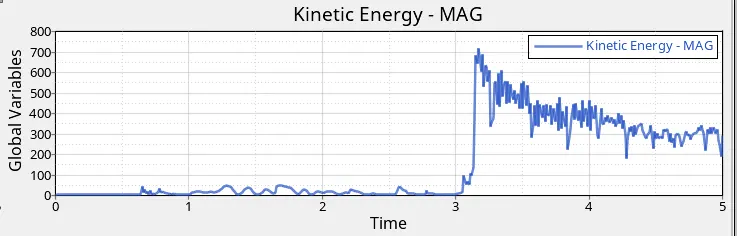
• Similarly in this case also most of the energy-storing is internal energy till plastic failure.
• After that elements break and start moving away since elements already have internal energy and when it loos the contact and start moving away all internal energy start converting into kinetic energy.

Total Energy-

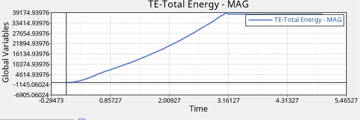
• The total energy is the sum of all types of energy present here, Kinetic+Internal+contact+hourglass.
• It will follow the same pattern as internal energy.

Comparison of all 7 cases-

Cases	Energy Error	Internal Energy	Kinetic Energy	External work	Mass Error	Elapsed time	Material used	Changed in material parameter	Element failure behavior
Case-1	0.8 %	0.2730*10^5	67.81	0.2721*10^5	0.0	108.56 s	Johnson cook [LAW2]	No change, Default shell parameters used and run.	Elements deleted
Case-2	4.1%	0.3082*10^5	141.9	0.2980*10^5	0.0	111.06 s	Johnson cook [LAW2]	change the value for lfail_sh, Dadv, Ixfem in failure card	Elements will crack and deleted
Case-3	0.8%	0.2744*10^5	87.08	0.2736*10^5	0.0	108.32 s	Johnson cook [LAW2]	Delete the failure card from the model browser.	Elements deleted
Case-4	1.1%	0.3879*10^5	3.931	0.3838*10^5	0.0	109.95 s	Johnson cook [LAW2]	Changed the maximum plastic strain value (Eps_max=0)	Elements deformed then cracked but not deleted.
Case-5	1.3%	0.8632*10^6	1677	0.8568*10^6	0.0	101.12 s	Elastic material [Law1]	Change the material card to law1 and run with the default parameter.	Elements deformed but not deleted.
Case-6	0.8%	0.2954*10^5	65.00	0.2940*10^5	0.0	110.68 s	Elasto plastic Brittle material [Law27]	Assign law27 and change the shell parameter. Also, assign rapture parameters for elements.	Elements break and Deleted.
Case-7	-2.3%	0.3606*10^5	369.0	0.3783*10^5	0.0	104.24 s	Elastic plastic Tabulated [Law36]	Created stress-strain using plastic strain and yield stress value. And also change shell parameters.	Elements break and Delete.

Result-

• Assigned all types of quality failure and shell parameters for all cases.
• Ran all the seven cases mode successfully and all created files were saved.
• Visualized all the models in hyper view. Plotted all the graphs in hypergraph-2D.
• Compared all the seven cases with their results.