Study and Comparison of different material laws

OBJECTIVE

Analysis and Comparison of different material laws used in Radioss.

PROCEDURE

a) Initial Setup:

i) Select Radioss from the user interface menu.

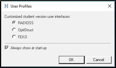
ii) First, we need to import the model into Hypermesh.

iii) To do so, click on Import -> Import Solver Deck -> Choose the starter file -> Import.

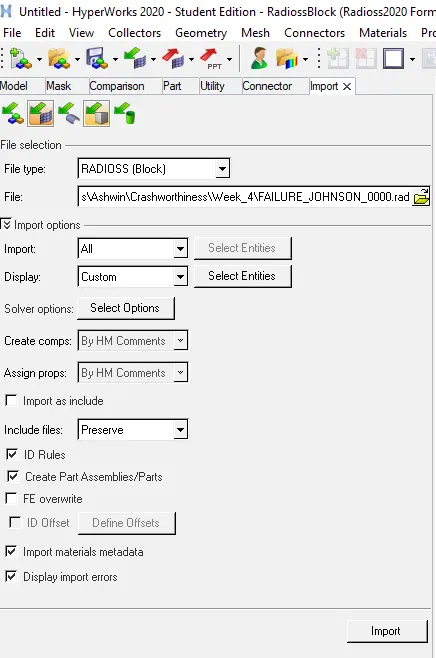
iv) After importing the following model is obtained:

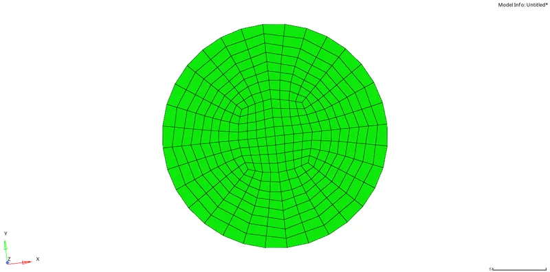
b) Case 1:

i) Run the simulation of the model without making any changes.

ii) To do the analysis, click on Analysis -> Radioss -> Select the file location and name -> Check 'include connectors' box -> Options = '-nt 4' -> Radioss.

[Note: When '-nt 4' is given in the options bar, the simulation will utilize 4 cores of the CPU thereby decreasing simulation time]

iii) To view the simulation, switch the menu to HyperView.

iv) Choose the required '.h3d' file from the simulation folder.

v) To plot the graphs we have to switch to HyperGraph 2D.

vi) Select the required T01 file from the simulation folder.

vii) To monitor the von mises stress in the simulation, click on Contour -> Result type=Von Mises(s) -> Averaging Method= Simple -> Apply.

viii) The following output is obtained:

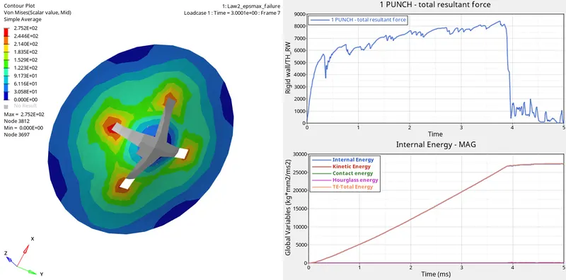
c) Case 2:

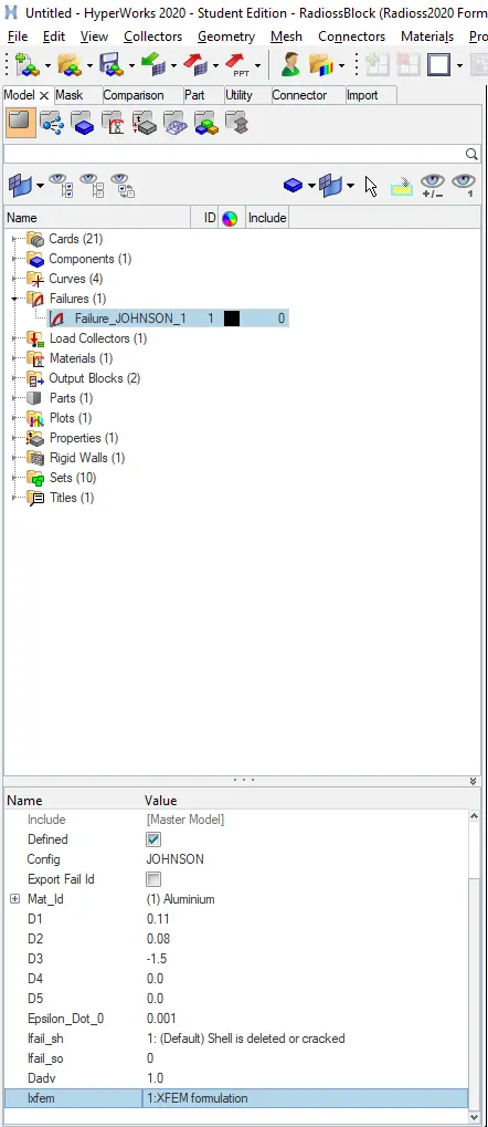
i) In /FAIL/JOHNSON card, change Ifail_sh=1,Dadv=1 and Ixfem=1.

ii) Follow the aforementioned procedure to run the simulation and plot the graphs.

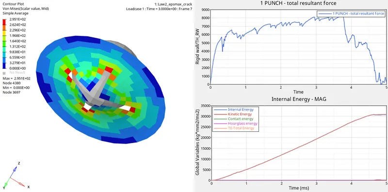
iii) The following output is obtained:

d) Case 3:

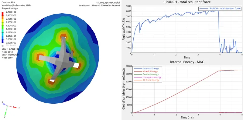
i) Delete the /FAIL/JOHNSON card and run the simulation.

ii) Follow the aforementioned procedure to run the simulation and plot the graphs.

iii) The following output is obtained:

e) Case 4:

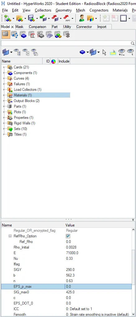
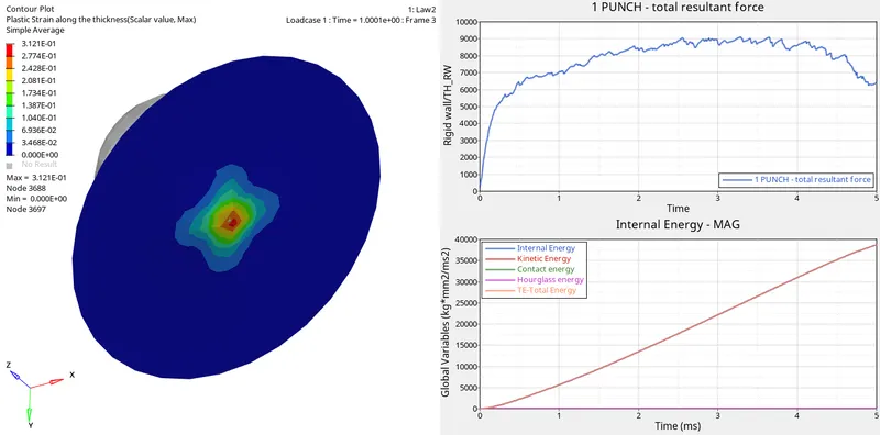
i) Delete the value of EPS_p_max and run the model.

ii) Follow the aforementioned procedure to run the simulation and plot the graphs.

iii) The following output is obtained:

f) Case 5:

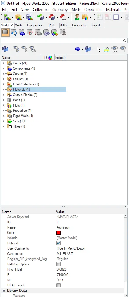
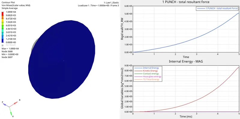
i) Change the material type to LAW 1 Elastic with the same Density(Rho_Initial), Young's Modulus(E) and Poisson's ratio(nu) values and run the model.

ii) Follow the aforementioned procedure to run the simulation and plot the graphs.

iii) The following output is obtained:

g) Case 6:

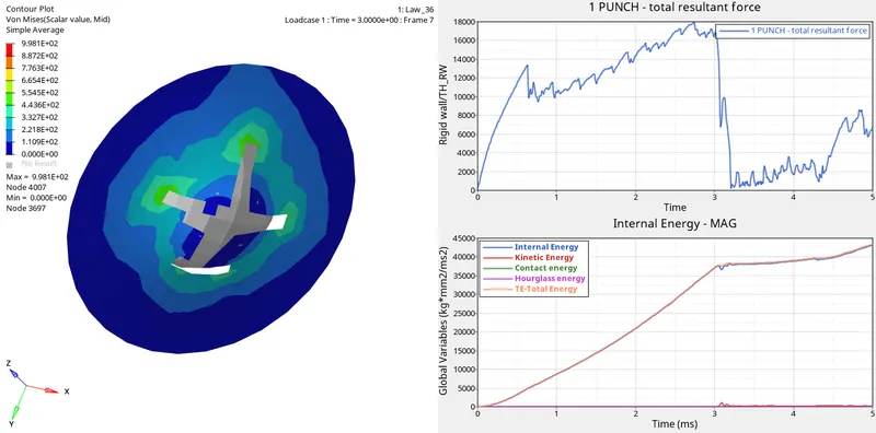
i) Change the material type to LAW 36 and run the model.

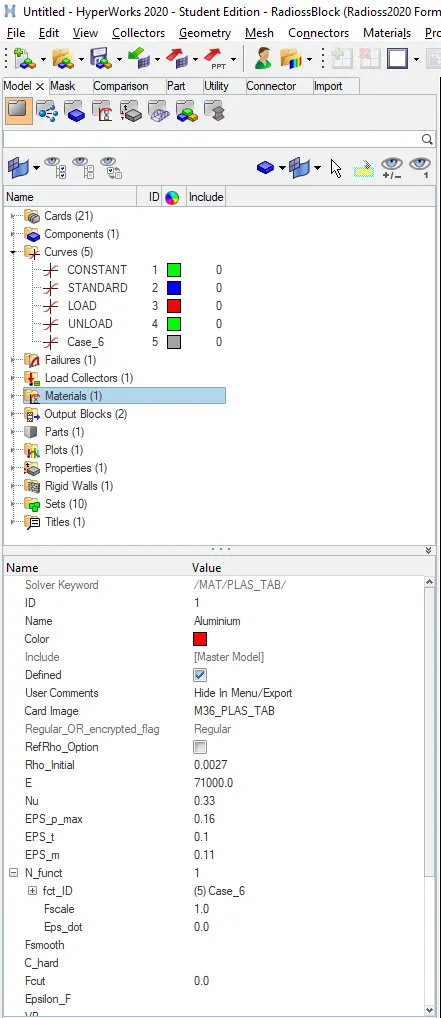
ii) Follow the aforementioned procedure to run the simulation and plot the graphs.

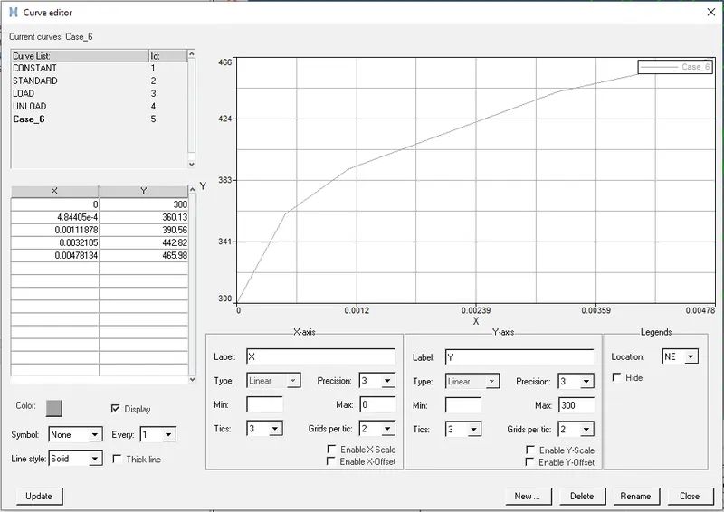
iii) The following graph shows the lab data curves:

iv) The following output is obtained:

h) Case 7:

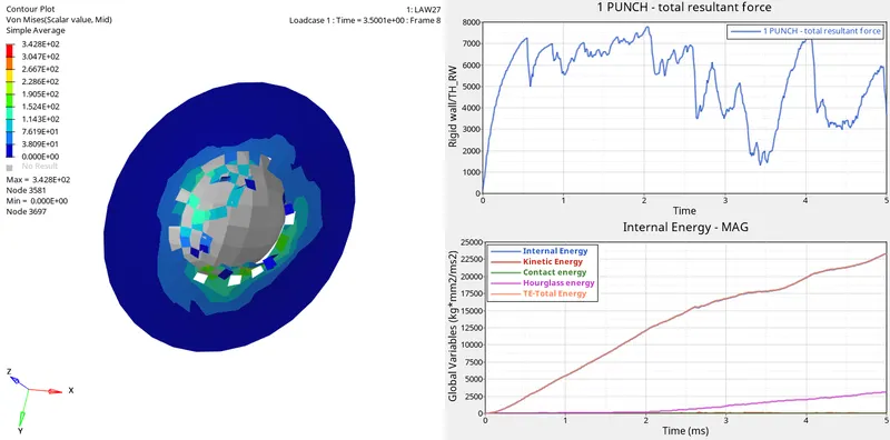
i) Change the material type to LAW 36 and run the model.

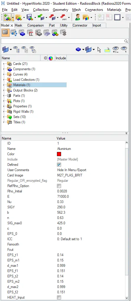
ii) Follow the aforementioned procedure to run the simulation and plot the graphs.

iii) The following output is obtained:

RESULTS

a) Case 1:

Sl. No	Name	Image	Observations
1.	Von Mises Stress		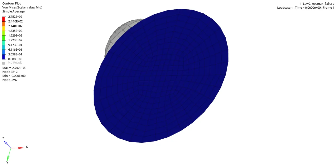The simulation represents the von mises stress present in the model. The Maximum Von Mises Stress obtained is 275 MPA. From the contour plot, we can see that the elements are getting deleted abruptly.
2.	Internal Energy		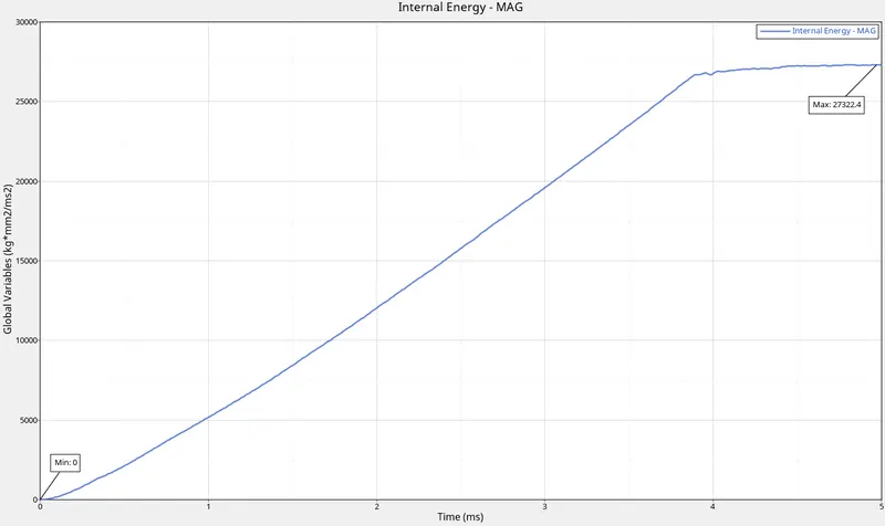The internal energy here represents the strain energy generated when the plate is deforming. Maximum Internal energy is 27322.4 kg*`mm^2`/`ms^2`
3.	Kinetic Energy		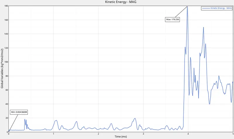Maximum Kinetic energy is 179.256 kg*`mm^2`/`ms^2`
4.	Contact Energy		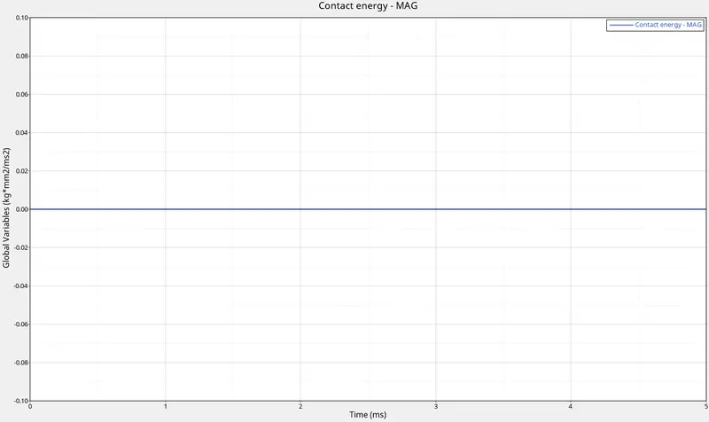Contact Energy is zero.
5.	Hourglass Energy		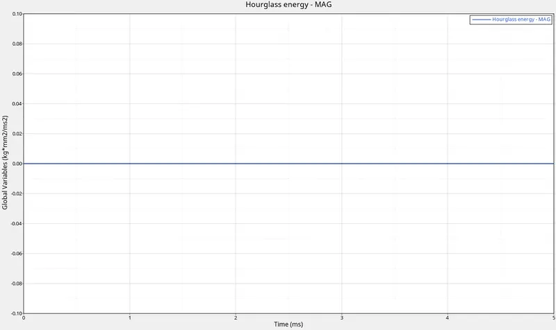Hourglass Energy is zero.
6.	Rigid Wall		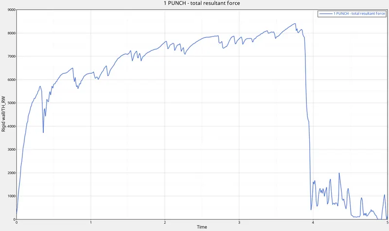The graph represents the forces endured by the rigid wall.
7.	Total Energy		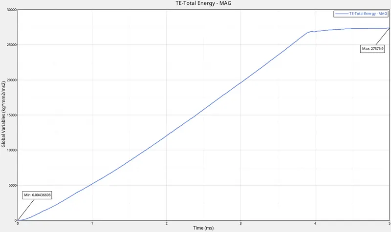The graph represents the total energy in the system.
8.	All Graphs		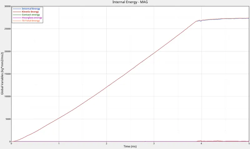The graph represents all the energies in the system.
9.	Energy and Mass error		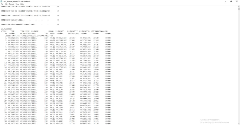Energy error is -0.3%. Mass added is zero. Both the values are within an acceptable range.
10.	Run Time		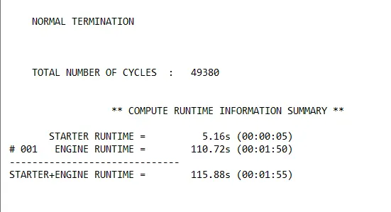Total run time= 115.88s(1:55 mins) Total number of cycles= 49380

b) Case 2:

Sl. No	Name	Image	Observations
1.	Von Mises Stress		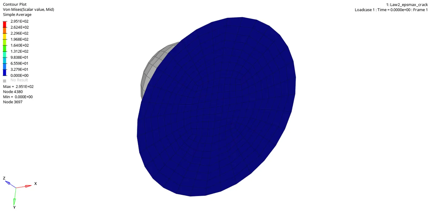The simulation represents the von mises stress present in the model. From the contour plot, we can see that the elements are getting cracked and then deleted. This is due to the new values given to the Johnson card. Ifxem=1 is used to see the cracking of elements when failure strain is reached by elements. Dadv is used to see crack advancement. The Maximum Von Mises Stress obtained is 295 MPA. We see a higher stress value compared to the previous case because the elements are failing only after cracking first. The key difference between the first and second cases is the cracking of the elements in the second one.
2.	Internal Energy		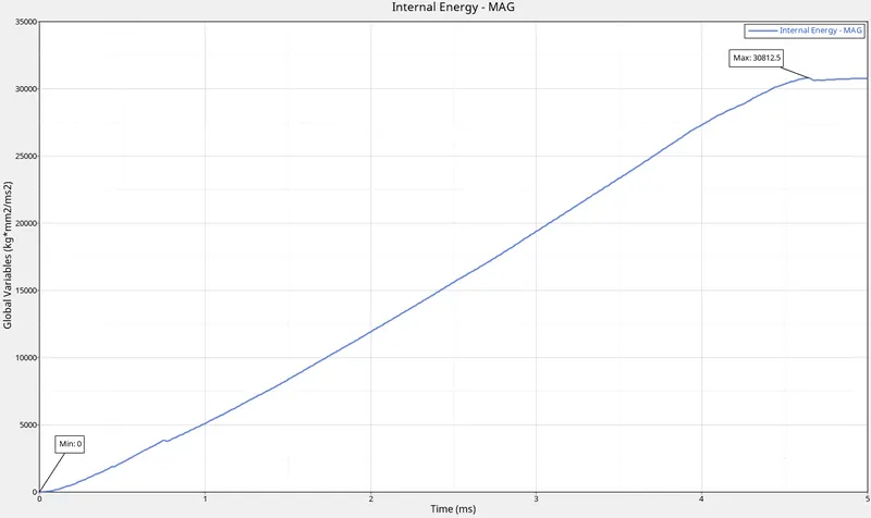The internal energy here represents the strain energy generated when the plate is deforming. Maximum Internal energy is 30812.5 kg*`mm^2`/`ms^2`. This model has more internal energy compare to the previous case.
3.	Kinetic Energy		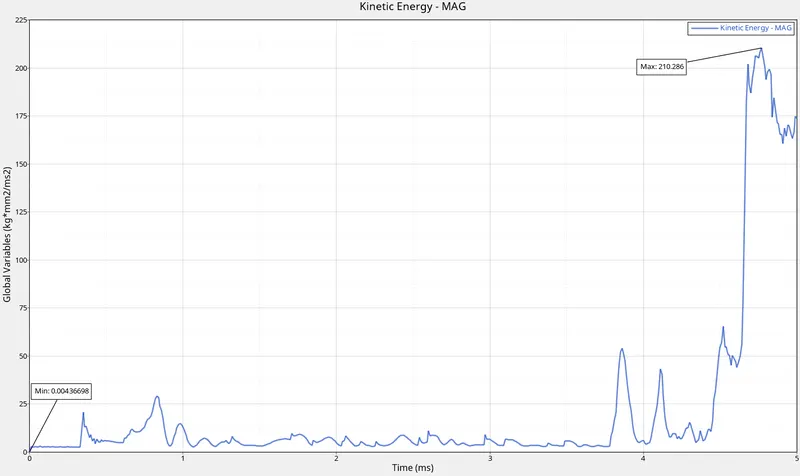Maximum Kinetic energy is 210.286 kg*`mm^2`/`ms^2` This model has more kinetic energy compared to the previous case.
4.	Contact Energy		Contact Energy is zero.
5.	Hourglass Energy		Hourglass Energy is 0.
6.	Rigid Wall		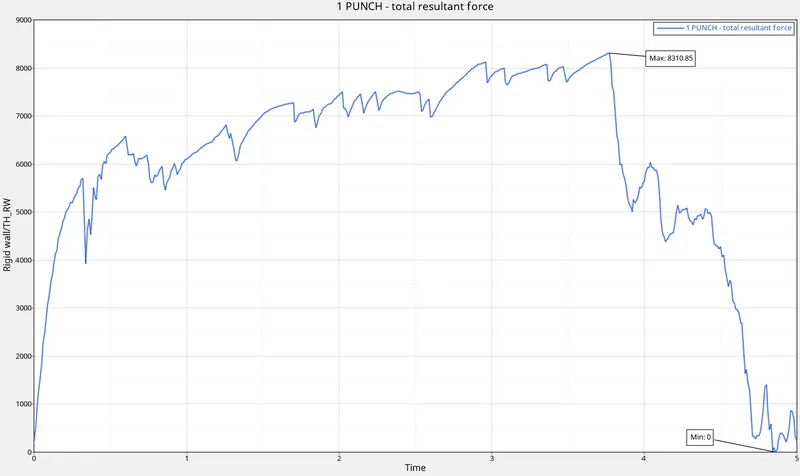The graph represents the forces endured by the rigid wall.
7.	Total Energy		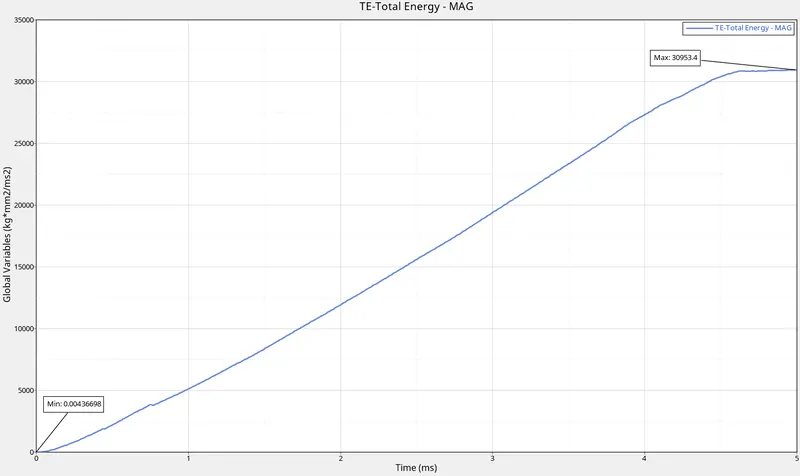The graph represents the total energy in the system.
8.	All Graphs		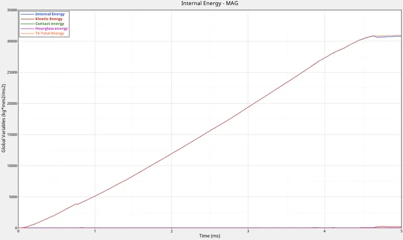The graph represents all the energies in the system.
9.	Energy and Mass error		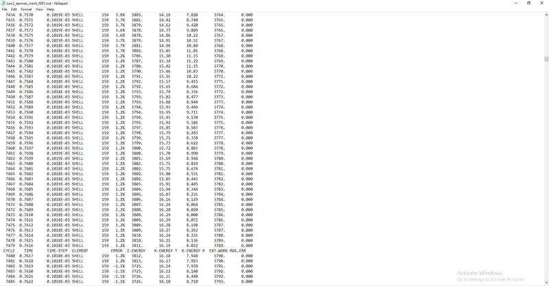Energy error is 4.5%. Mass added is zero. Both the values are within an acceptable range.
10.	Run Time		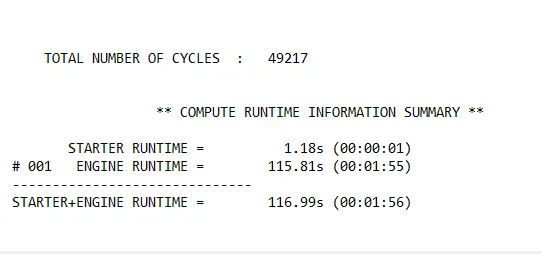Total run time= 116.99s(1:56 mins) Total number of cycles= 49217

c) Case 3:

Sl. No	Name	Image	Observations
1.	Von Mises Stress		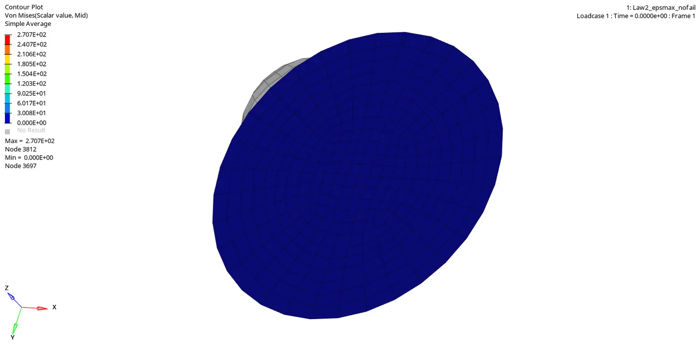The simulation represents the von mises stress present in the model. From the contour plot, we can see that the elements are getting deleted abruptly due to the absence of a failure model. This case is similar to the first one as the element gets deleted when it reaches maximum plastic strain. The Maximum Von Mises Stress obtained is 270 MPA. The von mises stress obtained is slightly lower than in the first case.
2.	Internal Energy		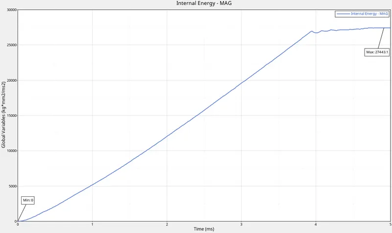The internal energy here represents the strain energy generated when the plate is deforming. Maximum Internal energy is 27443.1 kg*`mm^2`/`ms^2`
3.	Kinetic Energy		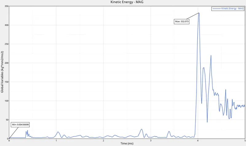Maximum Kinetic energy is 332 kg*`mm^2`/`ms^2`
4.	Contact Energy		Contact Energy is zero.
5.	Hourglass Energy		Hourglass Energy is zero.
6.	Rigid Wall		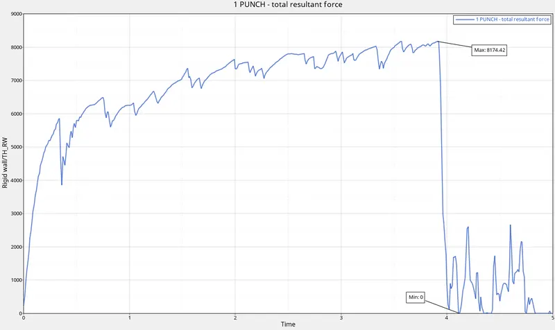The graph represents the forces endured by the rigid wall.
7.	Total Energy		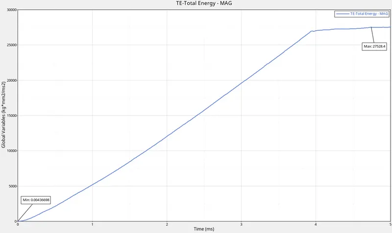The graph represents the total energy in the system.
8.	All Graphs		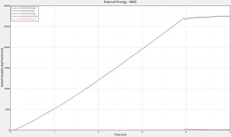The graph represents all the energies in the system.
9.	Energy and Mass error		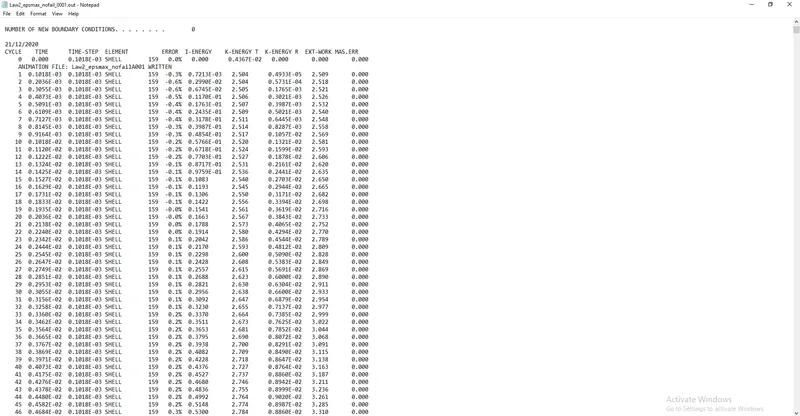Energy error is -0.3%. Mass added is zero. Both the values are within an acceptable range.
10.	Run Time		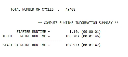Total run time= 107.92s(1:47 mins) Total number of cycles= 49408

d) Case 4:

Sl. No	Name	Image	Observations
1.	Von Mises Stress		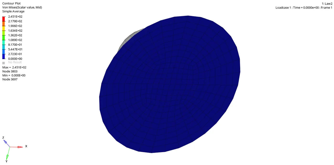The simulation represents the von mises stress present in the model. The Maximum Von Mises Stress obtained is 245 MPA.
2.	Internal Energy		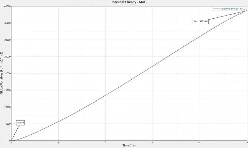The internal energy here represents the strain energy generated when the plate is deforming. Maximum Internal energy is 38724.8 kg*`mm^2`/`ms^2`
3.	Kinetic Energy		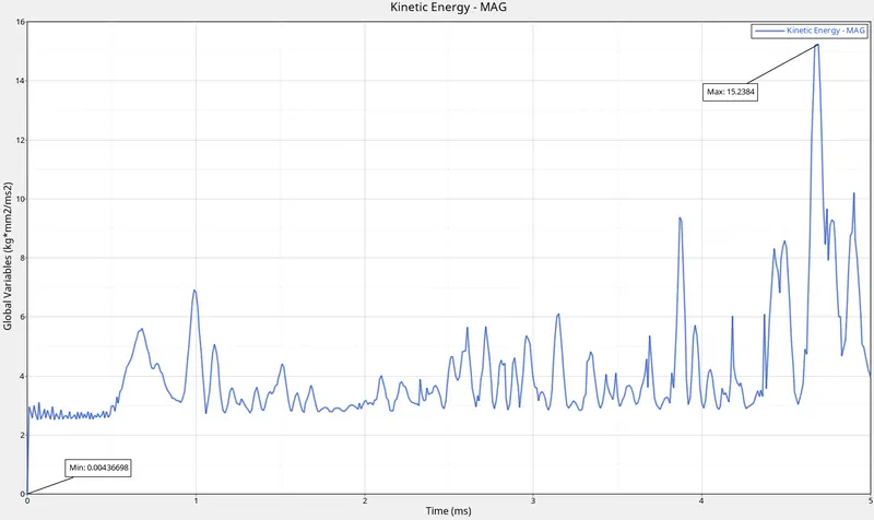Maximum Kinetic energy is 15.23 kg*`mm^2`/`ms^2`
4.	Contact Energy		Contact Energy is zero.
5.	Hourglass Energy		Hourglass Energy is zero.
6.	Rigid Wall		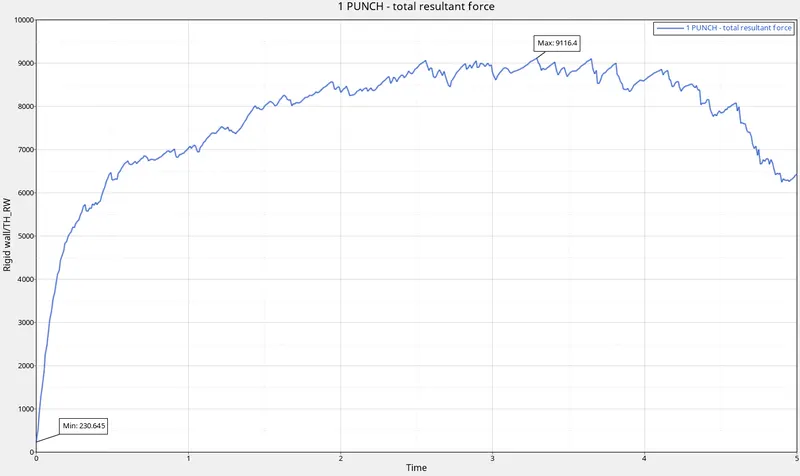The graph represents the forces endured by the rigid wall.
7.	Total Energy		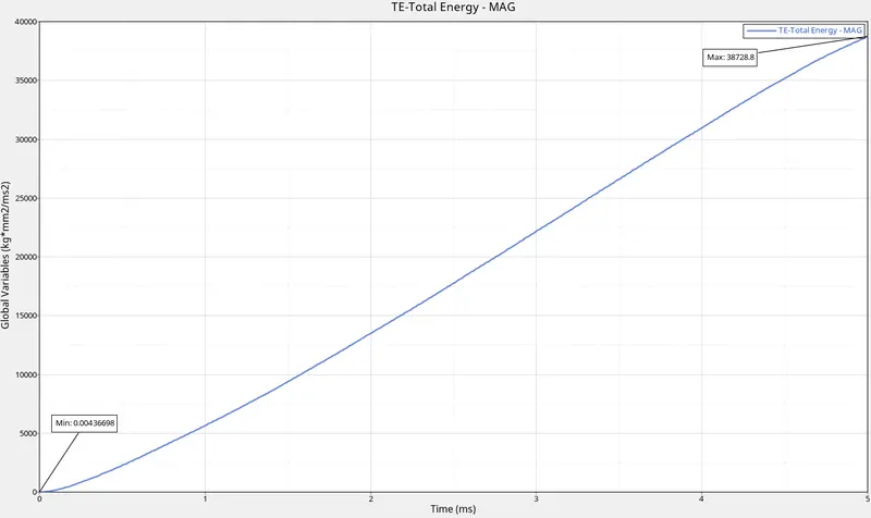The graph represents the total energy in the system.
8.	All Graphs		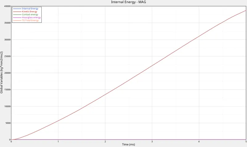The graph represents all the energies in the system.
9.	Energy and Mass error		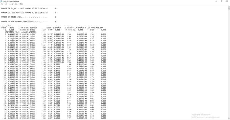Energy error is -0.3%. Mass added is zero. Both the values are within an acceptable range.
10.	Run Time		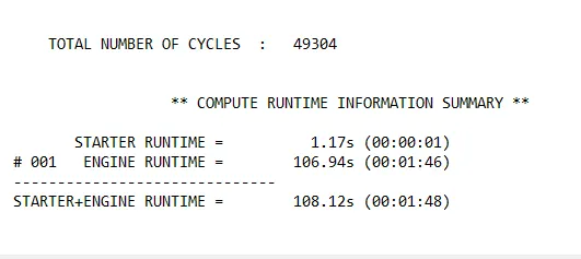Total run time= 88s(1:55 mins) Total number of cycles=49380

e) Case 5:

Sl. No	Name	Image	Observations
1.	Von Mises Stress		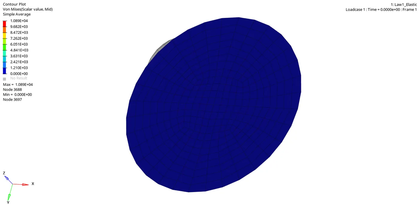The simulation represents the von mises stress present in the model. The Maximum Von Mises Stress obtained is 10800 MPA. The von mises stress is very high due to the constant deformation and increase in strain energy which in turn means high internal energy. This is due to the elastic nature of the material.
2.	Internal Energy		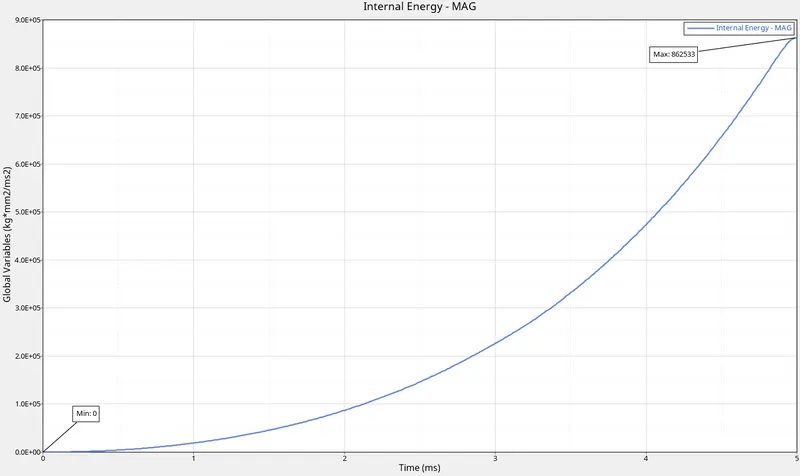The internal energy here represents the strain energy generated when the plate is deforming. Maximum Internal energy is 862533 kg*`mm^2`/`ms^2`.
3.	Kinetic Energy		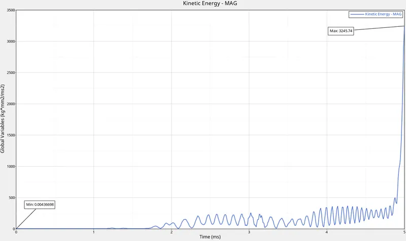Maximum Kinetic energy is 3245.74 kg*`mm^2`/`ms^2`.
4.	Contact Energy		Contact Energy is zero.
5.	Hourglass Energy		Hourglass Energy is zero.
6.	Rigid Wall		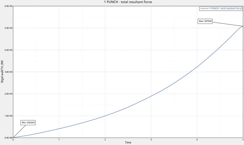The graph represents the forces endured by the rigid wall.
7.	Total Energy		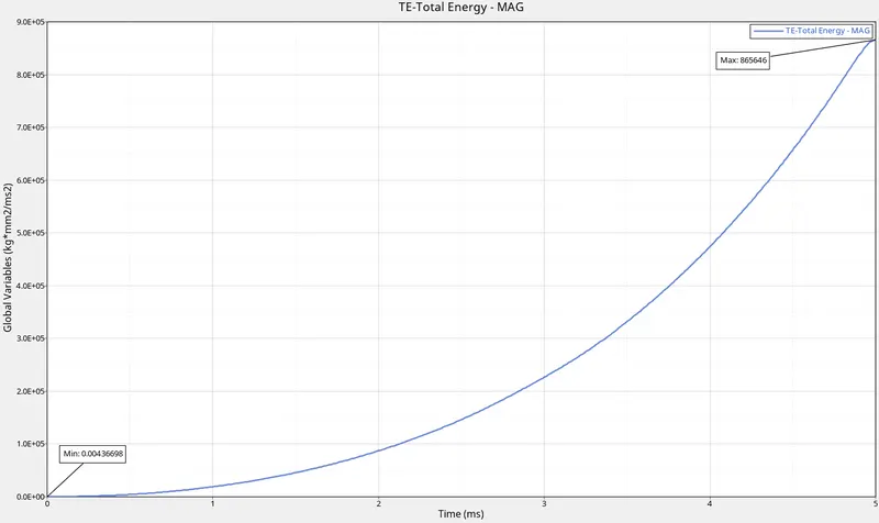The graph represents the total energy in the system.
8.	All Graphs		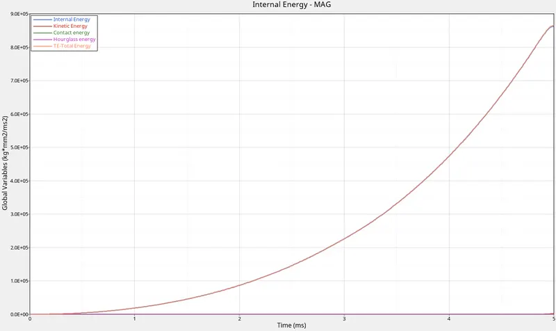The graph represents all the energies in the system.
9.	Energy and Mass error		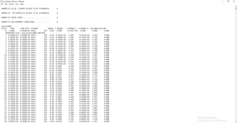Energy error is -0.3%. Mass added is zero. Both the values are within an acceptable range.
10.	Run Time		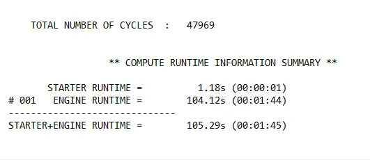Total run time= 105s(1:45 mins) Total number of cycles= 47967

f) Case 6:

Sl. No	Name	Image	Observations
1.	Von Mises Stress		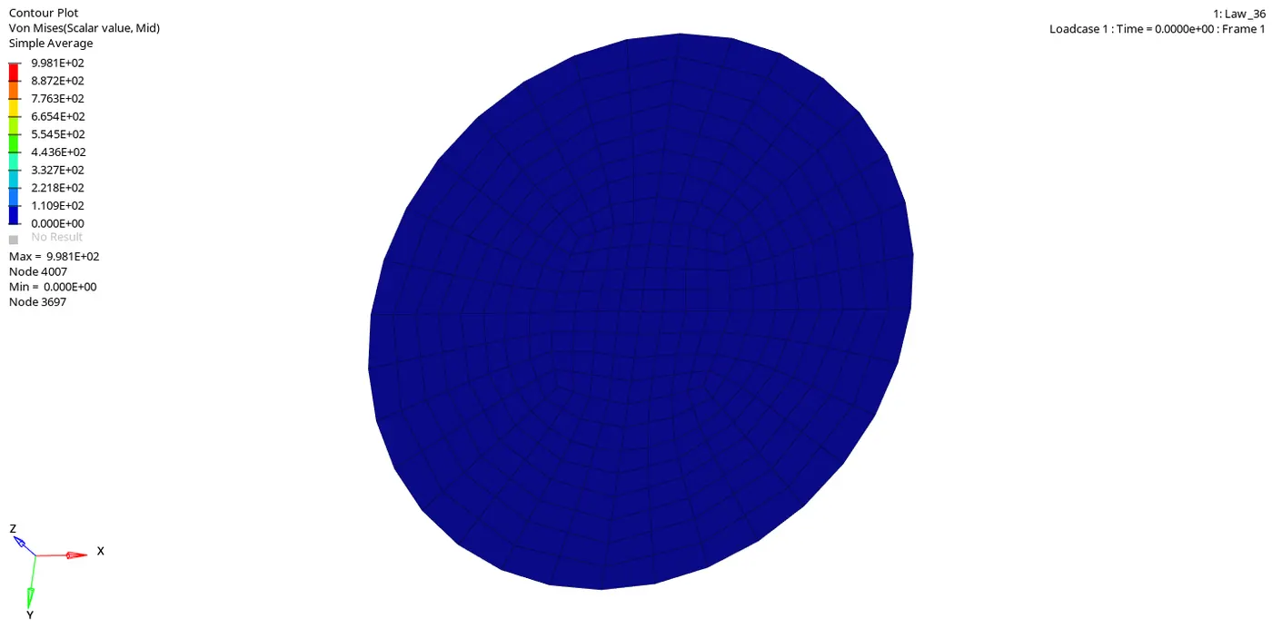The simulation represents the von mises stress present in the model. The Maximum Von Mises Stress obtained is 998 MPA.
2.	Internal Energy		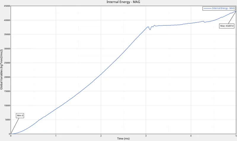The internal energy here represents the strain energy generated when the plate is deforming. Maximum Internal energy is 43207 kg*`mm^2`/`ms^2`
3.	Kinetic Energy		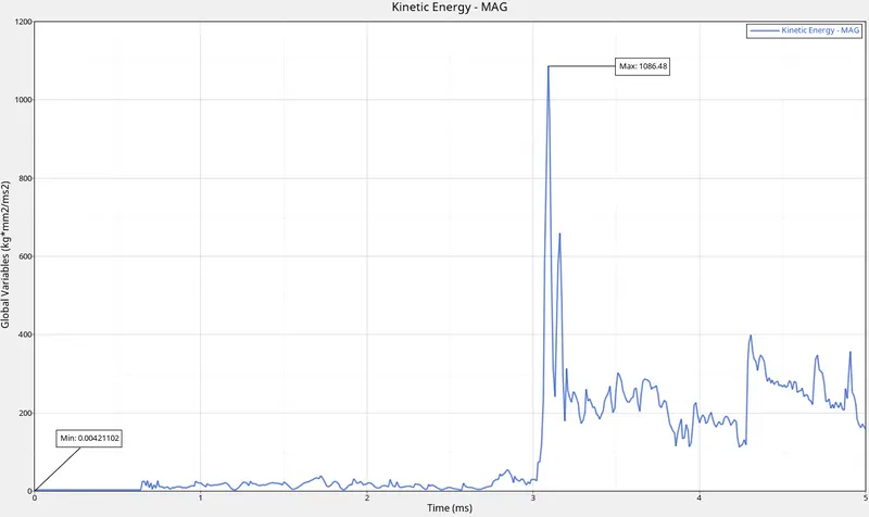Maximum Kinetic energy is 1086.5 kg*`mm^2`/`ms^2`.
4.	Contact Energy		Contact Energy is zero.
5.	Hourglass Energy		Hourglass Energy is zero.
6.	Rigid Wall		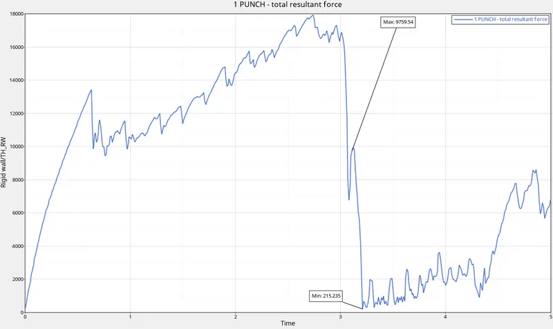The graph represents the forces endured by the rigid wall.
7.	Total Energy		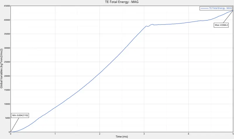The graph represents the total energy in the system.
8.	All Graphs		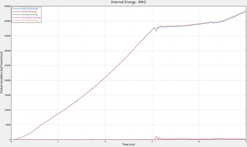The graph represents all the energies in the system.
9.	Energy and Mass error		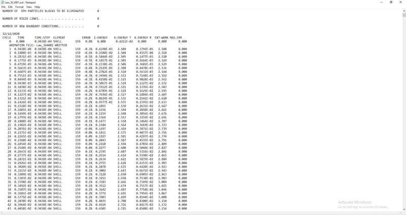Energy error is -0.3%. Mass added is zero. Both the values are within an acceptable range.
10.	Run Time		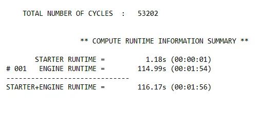Total run time= 116.17s(1:56 mins) Total number of cycles=53202

g) Case 7:

Sl. No	Name	Image	Observations
1.	Von Mises Stress		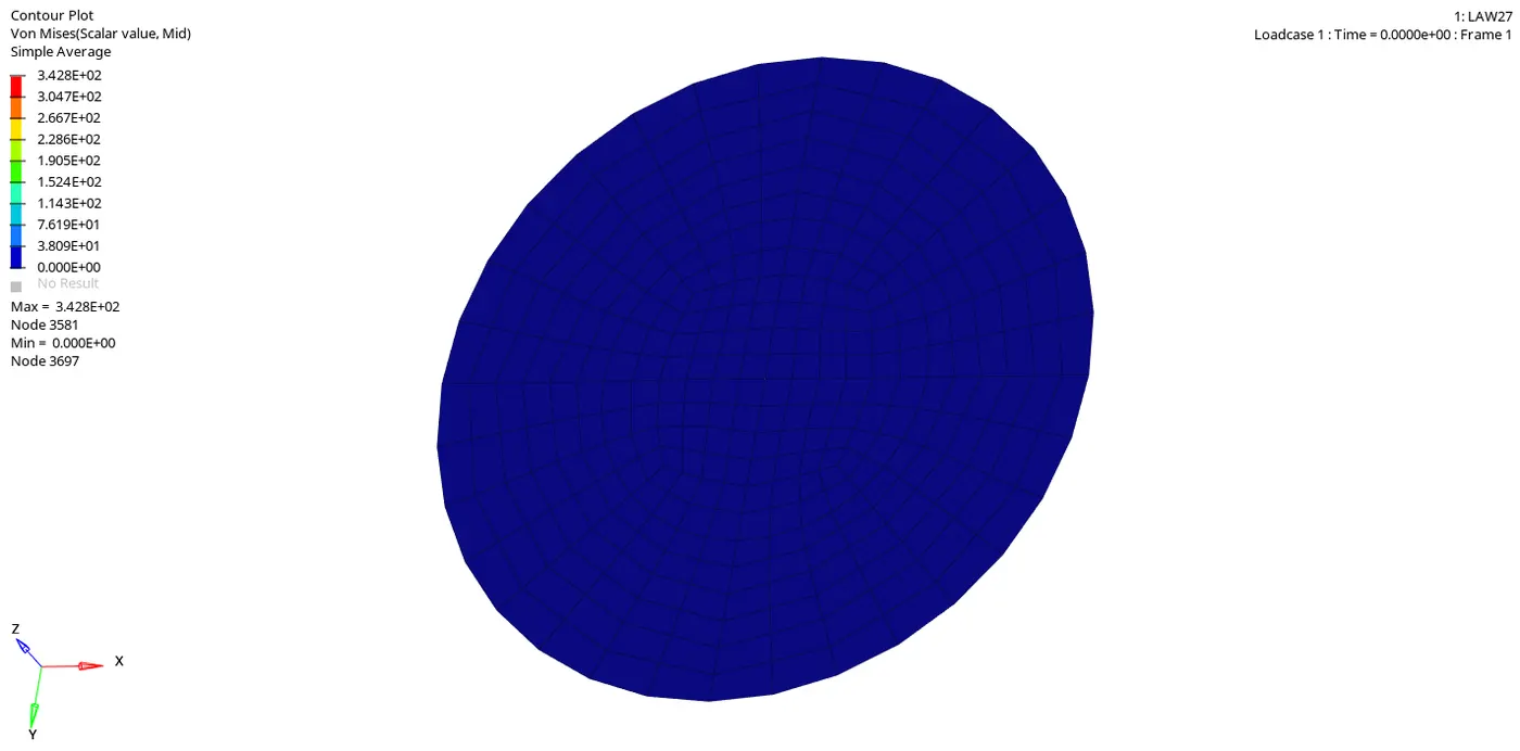The simulation represents the von mises stress present in the model. The Maximum Von Mises Stress obtained is 342 MPA. Failure and damage will occur only in tension. Simulation represents the brittle nature of the material.
2.	Internal Energy		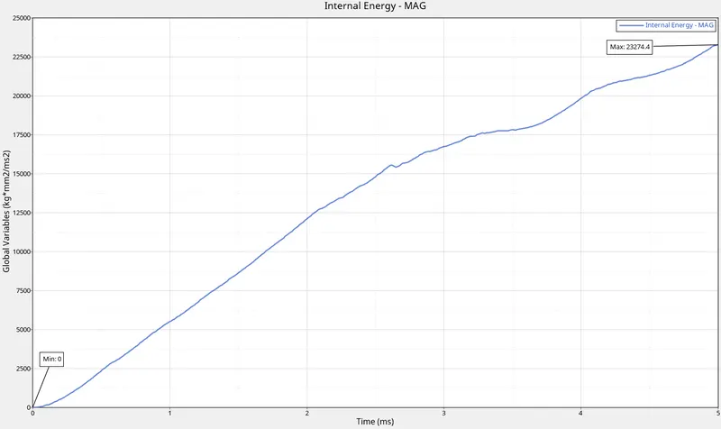The internal energy here represents the strain energy generated when the plate is deforming. Maximum Internal energy is 23274 kg*`mm^2`/`ms^2`
3.	Kinetic Energy		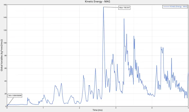Maximum Kinetic energy is 156.5 kg*`mm^2`/`ms^2`.
4.	Contact Energy		Contact Energy is zero.
5.	Hourglass Energy		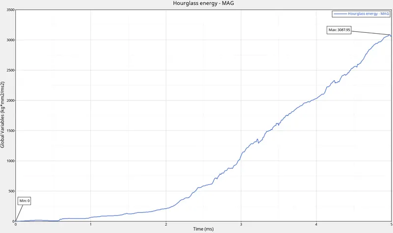Hourglass Energy is zero.
6.	Rigid Wall		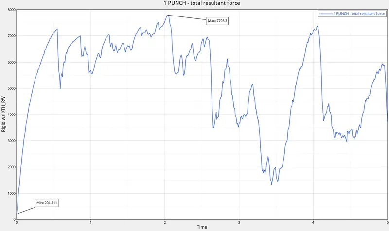The graph represents the forces endured by the rigid wall.
7.	Total Energy		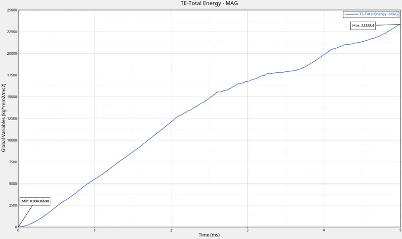The graph represents the total energy in the system.
8.	All Graphs		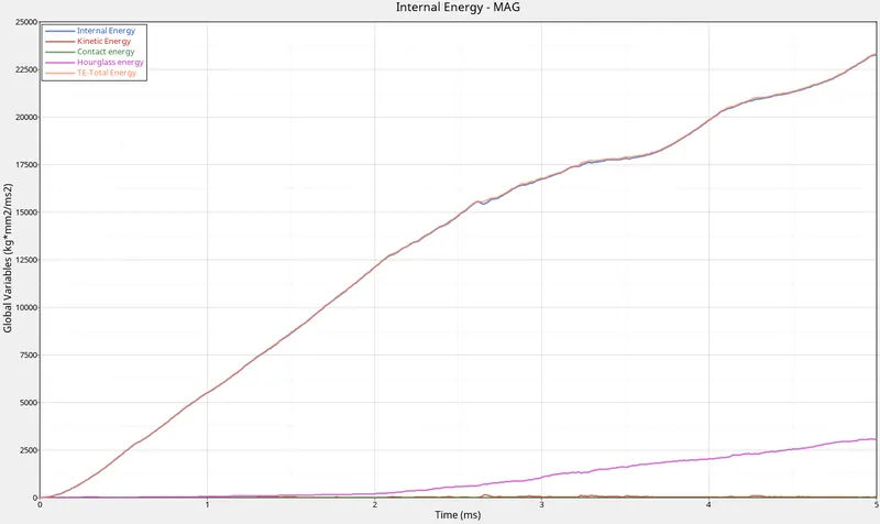The graph represents all the energies in the system.
9.	Energy and Mass error		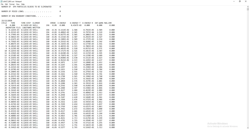Energy error is -0.3%. Mass added is zero. Both the values are within an acceptable range.
10.	Run Time		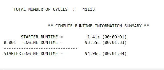Total run time= 94.96s(1:34 mins) Total number of cycles=41113

CONCLUSION

i) Selection of materials depends on the application.

ii) In a crash analysis, we prefer to use materials that will deform plastically by absorbing a lot of energy thereby decreasing occupant injury.

iii) Based on the results, we can conclude that Lawe 36 is found to best suited for the current application.

iv) It replicates the material used in real-time situations.

v) We can directly input the stress-strain curve obtained from lab results.