Assignment 4

• Objective: Using different material models, perform the simulation on the rupture plate and compare the results.
• Case 1: Law2 material model with Eps_max failure mode

Import the given component. Go to File > Import > Solver Deck. Click on open file icon and navigate to the folder where file is stored and click on open after selecting the file. Now click on Import. The

setup will be imported as seen below. The shell elements properties are checked and are found well defined to the recommended values. Also the material properties - yield stress, hardening modulus

and hardening exponent are well defined in the material model along with other required properties. We can directly run the analysis.

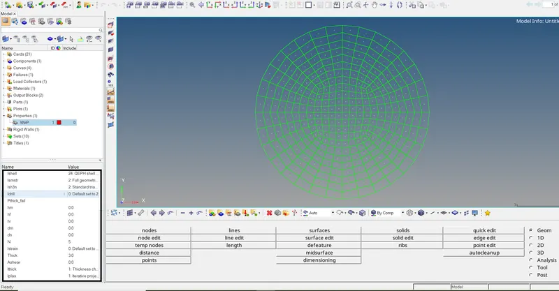
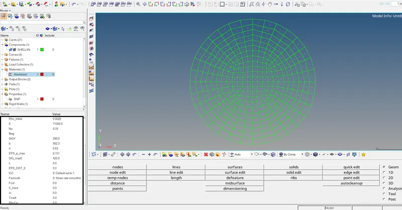
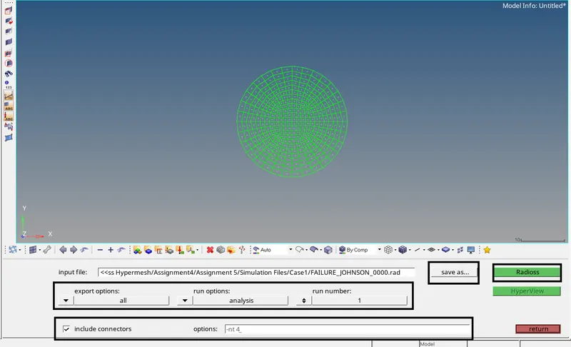
To run the analysis, go to Analysis > Radioss. In the save as option, give the path to save the file and click on Radioss. The solver will start the analysis.

Case 2: In case2 we have to make changes in the Johnson cook failure card. Edit the values as follows:

Ifail_sh = 1, Dadv = 1 and Ixfem = 1.

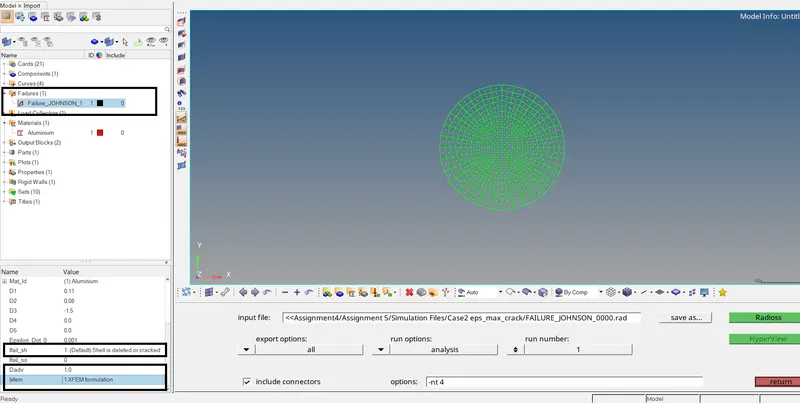
As discussed earlier, repeat the same process to run the simulation.

Case3: In case3, we have to delete the Johnson cook failure card.

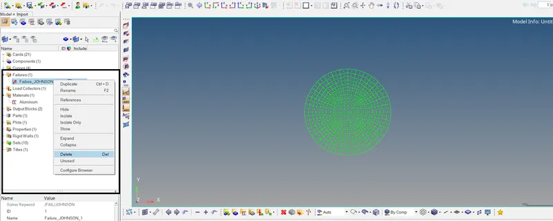
After deleting the failure card, run the simulation.

Case4: In this case, we have to delete the value of Eps_max (Eps_max = 0) and run the simulation.

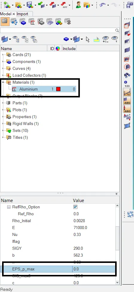
Case5: Here, we have to change the Law2 material model to Law1 (Isotropic Linear Elastic). Change the Card Image to M1_ElAST and enter the values for E, nu and density. Then run the simulation.

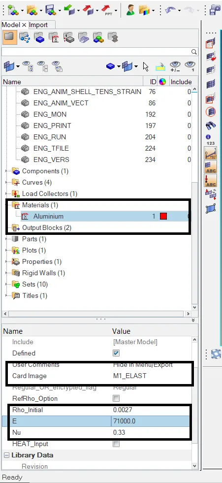
Case6: Here, we have to convert the material model into Law36. In the material collector, click on the material name. Change the Card Image to M36_PLAS_TAB. Enter the values for E, nu and density for

aluminium. Enter Eps_max = 0.16, Eps_t =0.1 and Eps_m = 0.11. Using Mat36, we can define the stress strain curve for the material. To create stress-strain curve, right click on Curves in the modal view

and click on create. Name the curve as Law36. Enter the following values of stress-strain and click on update. The curve will be generated.

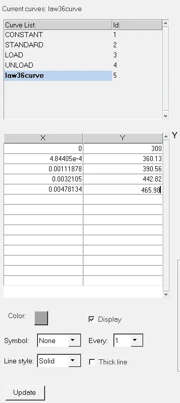
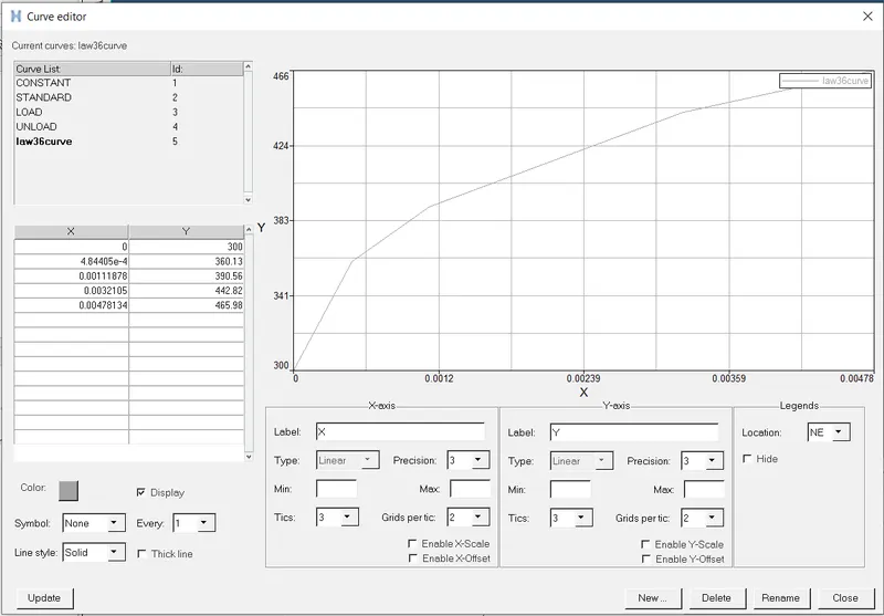
Update the given material with this curve. Click on the material name in the material collector. Enter N_funct = 1 and in fct_ID select law36 curve.

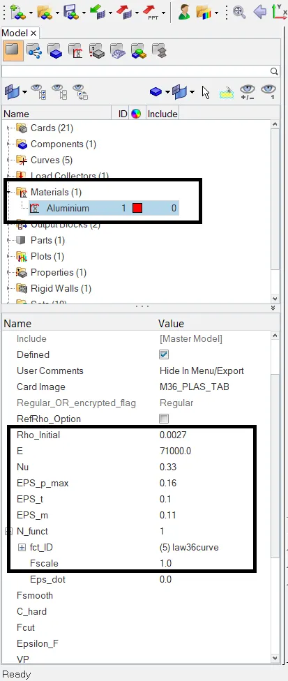
Now run the simulation.

Case7: Import the Law27_0000.rad file. There are no properties well defined for shell elements. Enter the recommended values for the properties.

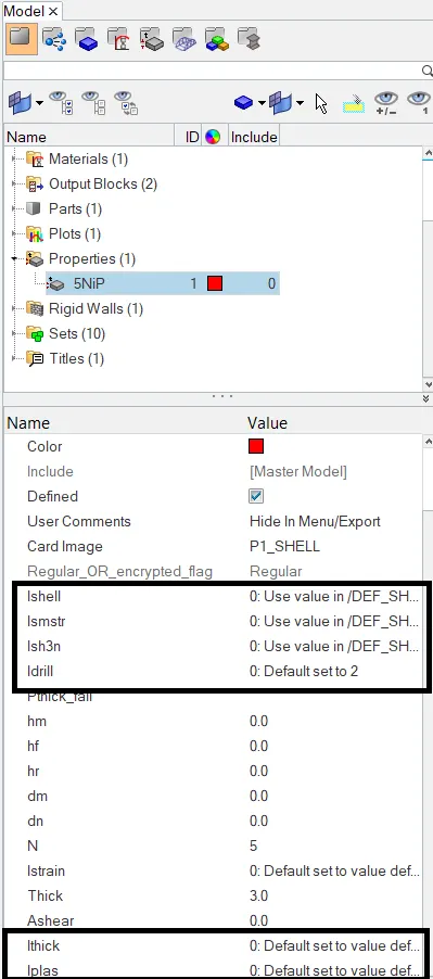
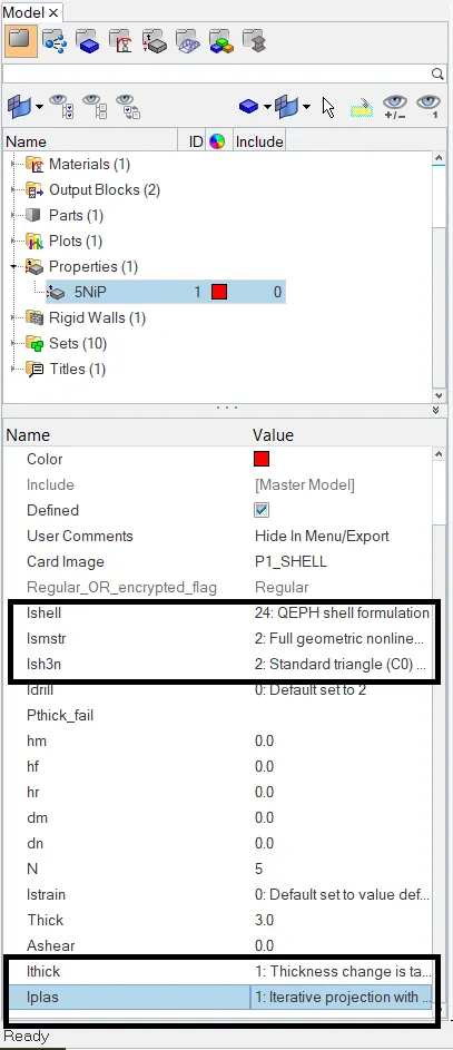
All other parameters are defined and we can run the simulation.

• Comparison of cases:

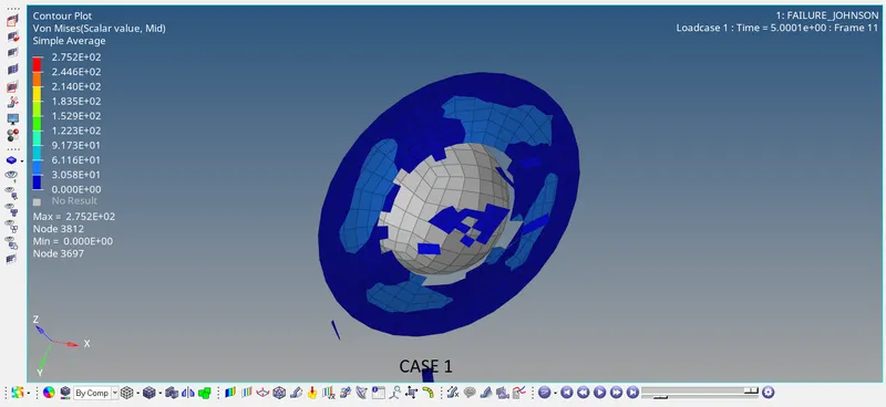
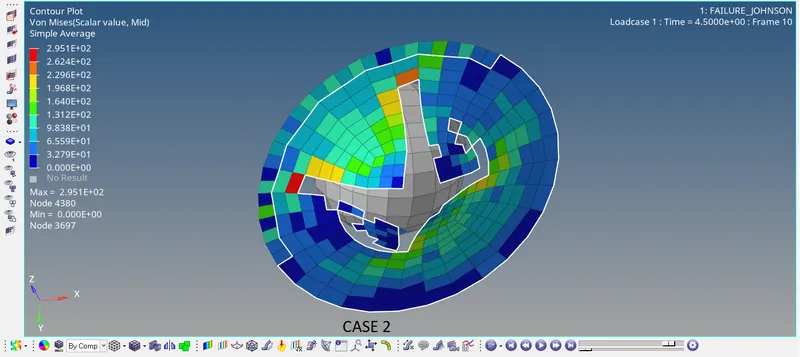
Both case 1 and case 2 material are isotropic elasto plastic materials modelled using M2_PLAS_JOHNS card. Also failure card fail_JOHNSON is defined to consider the mode of deformation. D1, D2 and D3

values are defined. For case 1, the Ixfem parameter is set to 0 in the failure card. As a result, in case 1, no crack propogation is observed in the shell elements. The failing elements are deleted. Whereas,

in case 2, Ifail_sh = 1 will enable the element to either crack or to be deleted upon failing. Dadv =1 criteria will allow failing element for the crack advancement when Ixfem = 1. The crack propogation

is observed as seen above. In case 1, as the elements are getting deleted, more energy is dissipated and less stresses are developed. Whereas in case 2, the elements are getting cracked and less energy

energy is dissipated and the stress deveoped is more compared to case 1.

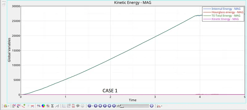
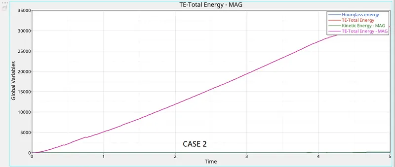
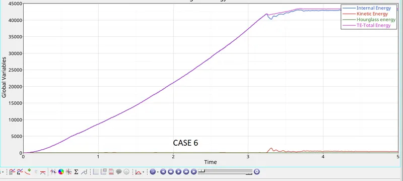
As seen in both cases, the internal energy increases linearly and then starts fluctuating after some time. It is indicative by the graph, internal energy increases linearly in the elastic region due to the

absorbtion of kinetic energy and starts fluctuating once it enters the plastic region.

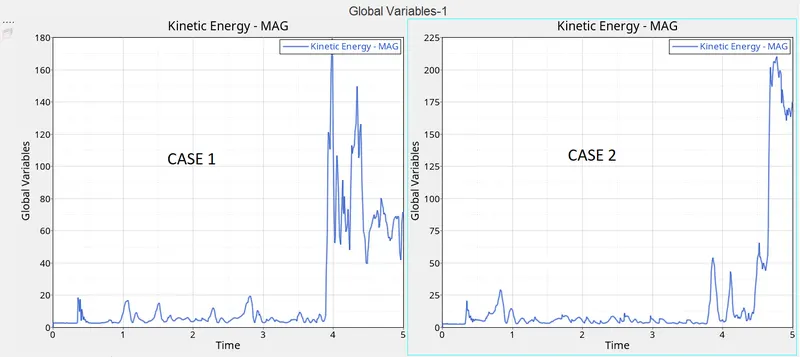
There is some noise in the graph of kinetic energy. This can be attributed to the elements being deleted after failure. Whereas in case 2, the fluctuation in graph of kinetic energy is less compared to case1.

Case 3 & 4:

In case 3, the fail_JOHNSON card is deleted. The elements fail, when one integration point reaches Eps_max and the failed elements are deleted similar to case 2. In case 4, the Eps_max is set to 0.

In this case, there is no plastic strain for failure defined. The elements will fail once the stress in the elements crosses the defined limit of 425 Mpa. As seen below, the induced stresses in the rupture

plate is less than 425 Mpa, the elements will continue to deform plastically resulting in more energy dissipation.

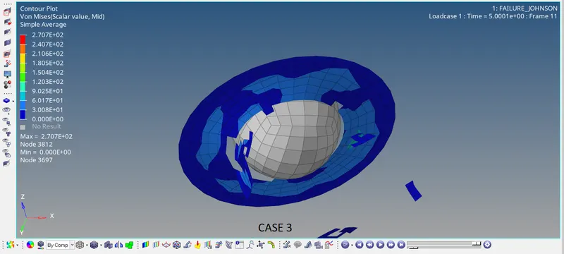
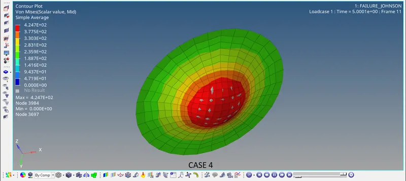
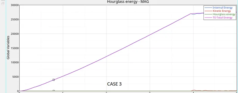
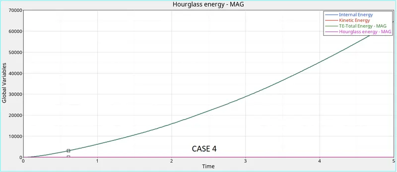
In both cases, the internal energy increases linearly due to the impact of sphere. The internal energy is more in case 4 due to more streching of the elements without failing compared to case 3.

Case 5 & 6:

In case 5, the case 4 model is converted into isotropic linear elastic model using M1_ELAST card. In case 6, case 5 model is converted into isotropic elasto plastic model using M36_PLAS_TAB card.

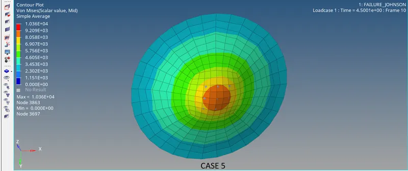
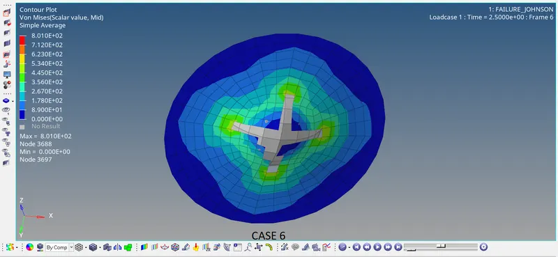
For case 5, plate behaves as an elastic material which will follow linear relationship between stress and strain obeying Hooke's law. It behaves as an elastic material and will never fail. Less energy

dissipation will be observed and the induced value of stress will be high. Whereas in case 6, plate will behave as an isotropic elasto plastic material. Epa_max is the defined rupture parameter and

the failed element will be deleted from the model as seen above.

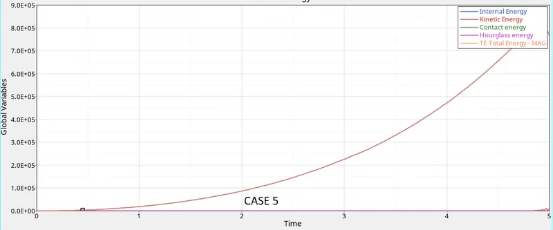
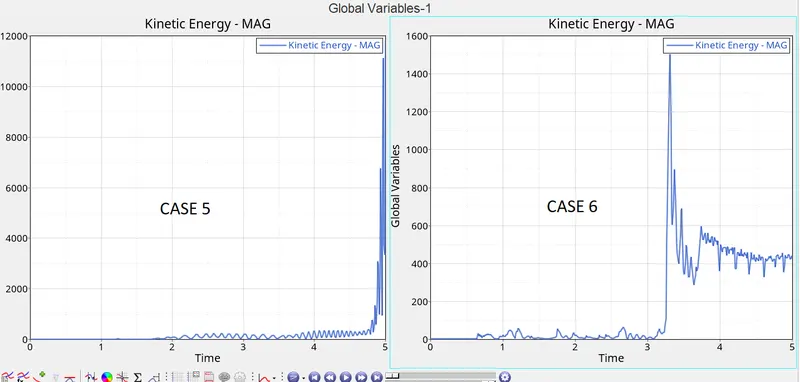
There is gradual increase in kinetic energy in case 5, due to streching of the elements due to elastic nature of the material. In case 6, sudden hike of the kinetic energy represents deletion of elements

due to failure of the element.

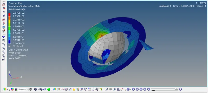
Case 7: In this case the PLAS_BRIT card is used. This card combines an isotropic elasto plastic Johnson cook material with an orthotropic brittle failure mode. The component behaves as an brittle material.

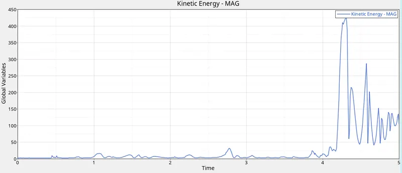
As seen below, the plate fails behaving like a brittle material like glass. A shattering like effect is observed. A huge spike in the kinetic energy can be observed. This spike corresponds to the failing

elements being deleted.

Comparing all the above material model, law 36 (PLAS_TAB) material model could yield realistic results, since we can define the stress-strain curve for different strain rate.Data can be obtained from lab

test and more accurate FE model can be created, which will give results close to experimental data since the behaviour of the material is expected to follow the real life behaviour observed in lab test.

• Conclusion: All simulations are performed according to the given conditions using different material model and comparison between them is made. The case to be used for solving this problem is

justified with reason.