Analysis for a Plate with different Material and Element Properties using RADIOSS.
Assignment 4 Report.
- Objective: To compare all the cases of Elemental Failure and Elemental Behaviour when we change the Element and the Material properties. We further study the effect in the change of Failure card and to tabulate certain criteria such as the Number of cycles, Hourglass energy etc for all the various cases that were peformed.
- Procedure: So we need to compare all the various cases of how the element fails when we change the properties according to the cases mentioned. Here is the detailed description of each and every case:
Case1: In this case we need to run the base Simulation. Before running this simulation, we need to change the Shell Elemental Properties to the recommended values. The following properties were used:
a. Ishell = 24 (QEPH with reduced Integrated elements.)
b. Ismstr = 2 (Full Geometric linearities with small strain formulation possible.)
c. Ish3n = 2 (Standard 3 noded Shell Element with large rotation.)
d. N = 5 (Number of Integration points.)
e. Ithick = 1 (Thickness change taken into account.)
f. Iplas = 1 (Iterative plasticity for good accuracy.)
The very first step when we have to change the run time in the model we need to firstly import the model. To import it, we need to click on the Import button and use the file option in it.
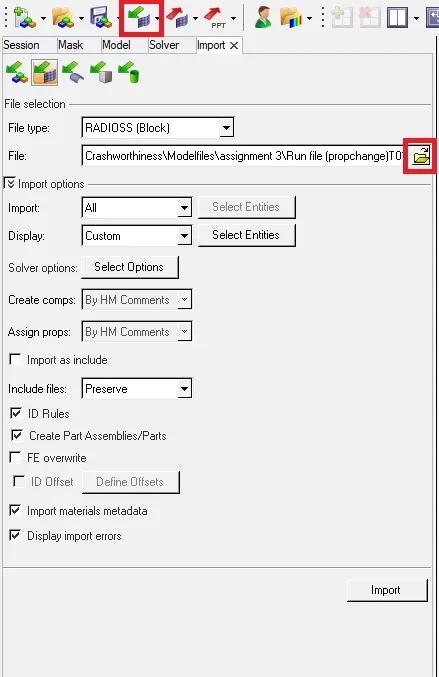
Import a model.
After we import the starter file, then we need to check the elemental properties and set them to the properties mentioned earlier. To check the Element Proerties, we need to click on the Properties card and change the properties to the required values.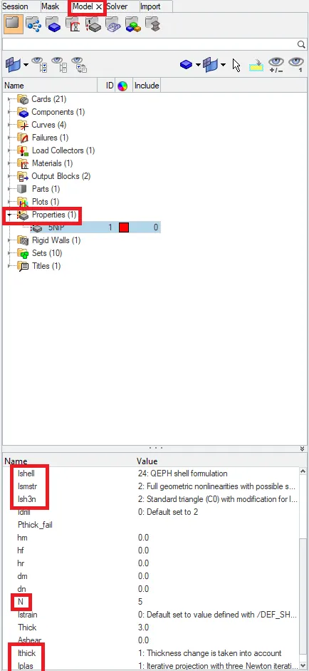
Property Change.
Here we need to change the values of the elemental properties as per the requirement. We can see that the elemental properties are changed according to the requirement.
After the properties were changed, we then need to run this simulation. To run this simulation, We need to use the RADIOSS command in the Analysis tab.
Analysis -> RADIOSS
RADIOSS command
After we run this simulation, we then need to analyse the simulation frame by frame and understand the plate properties with the elemental behaviour in the plate.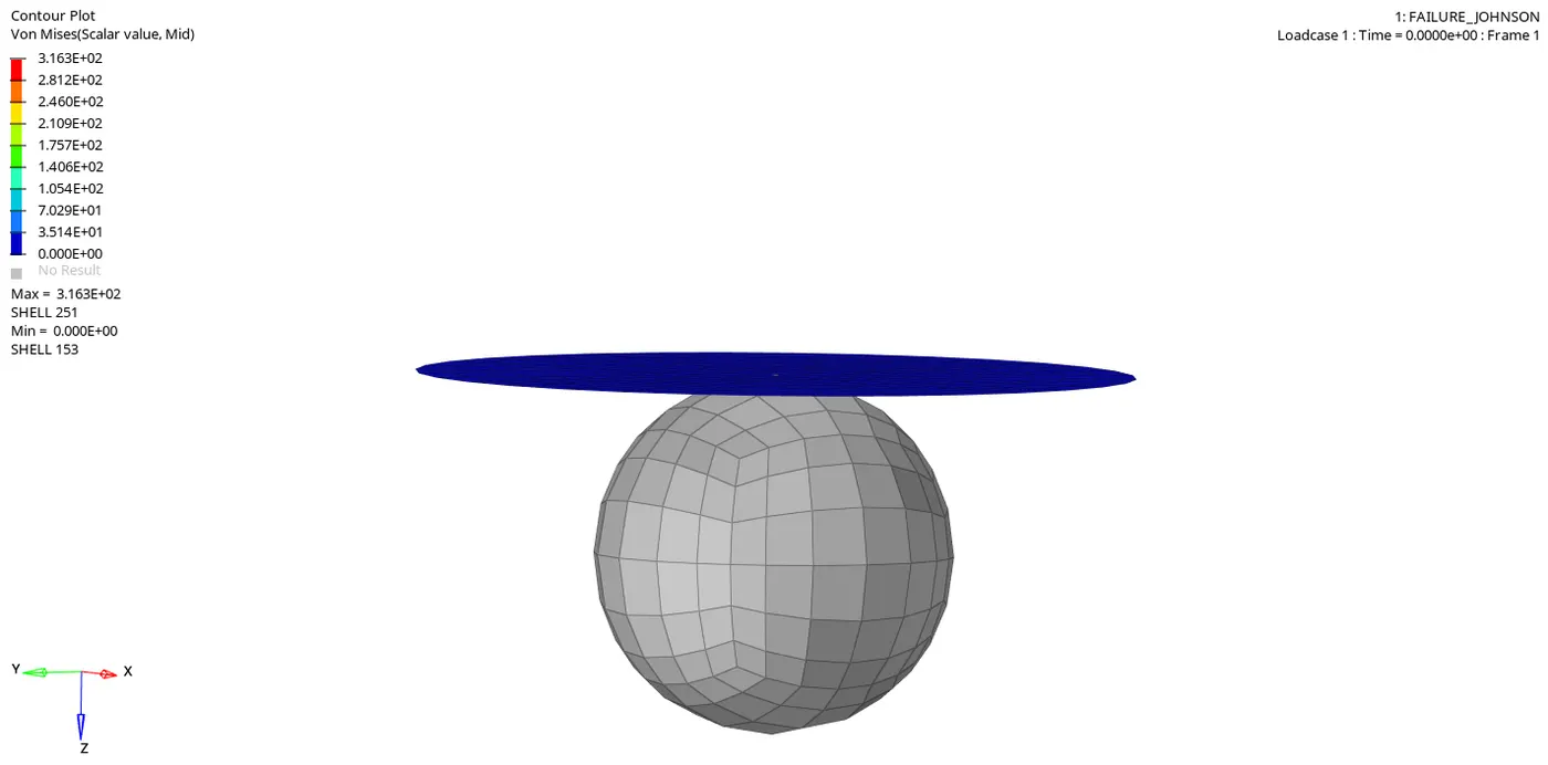
Simulation for Case1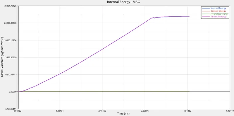
Graph Plot Case1
Case 2: In this case, we need to alter the values in the Failure card. To change these values, we need to click on theFailure card and change the following given values.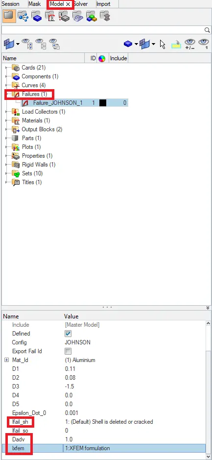
Changing the Failure Card Properties.
We need to change the values of Ifail_sh = 1 which determines the Shell element Failure method. So there are two ways in which we can see the element failing, the element will either get deleted or in some cases the cracking occurs according to the material properties.
There are two different Failure methods:
Element Rupture (Ixfem = 0)
Element Rupture (deleted) (if D>1)
The other value that was to be changed was, Dadv = 1 which indicates how the crack advancement will take plcae in the element. there are other values that we consider such as D1, D2, D3, D4, D5 when we change this value.The Value of D is dependent on the material and loading conditions set. So, these five values can be used to calculate the Value of D. If this value of D is greater than the Value of Dadv set, then the Crack advancement will occur according to the Dadv value. the element is deleted if a second crack is developed on it.
The next value to be changed is the value of Ixfem to 1. There are only two values in the Ixfem property, i.e 0 and 1. So if the Value of Ixfem is kept as 0, then the element will get deleted incase it fails. But, if the value of Ixfem is kept as 1, then the cracking along the meshed surfaces occurs. The Dadv value can only be used if the Ixfem is set to 1.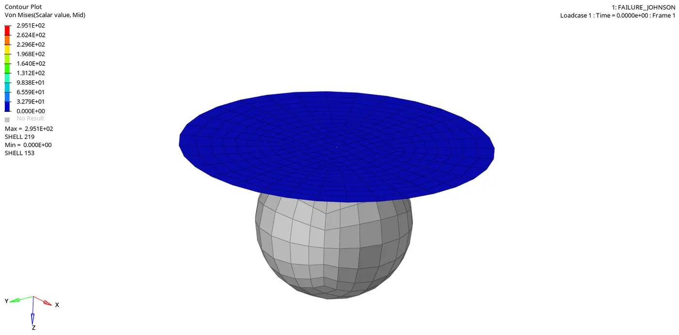
Simulation for Case 2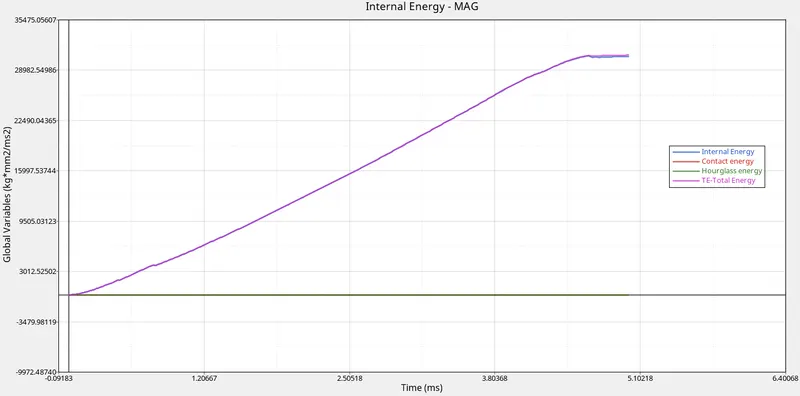
Graph for Case2
Case 3: In this case, we are supposed to delete the Failure card and then run the simulation. To delete this card, we simply need to right click on the failure card "Failure_JOHNSON_1" and then click on delete. Then we need to run this model and observe the graphs as well.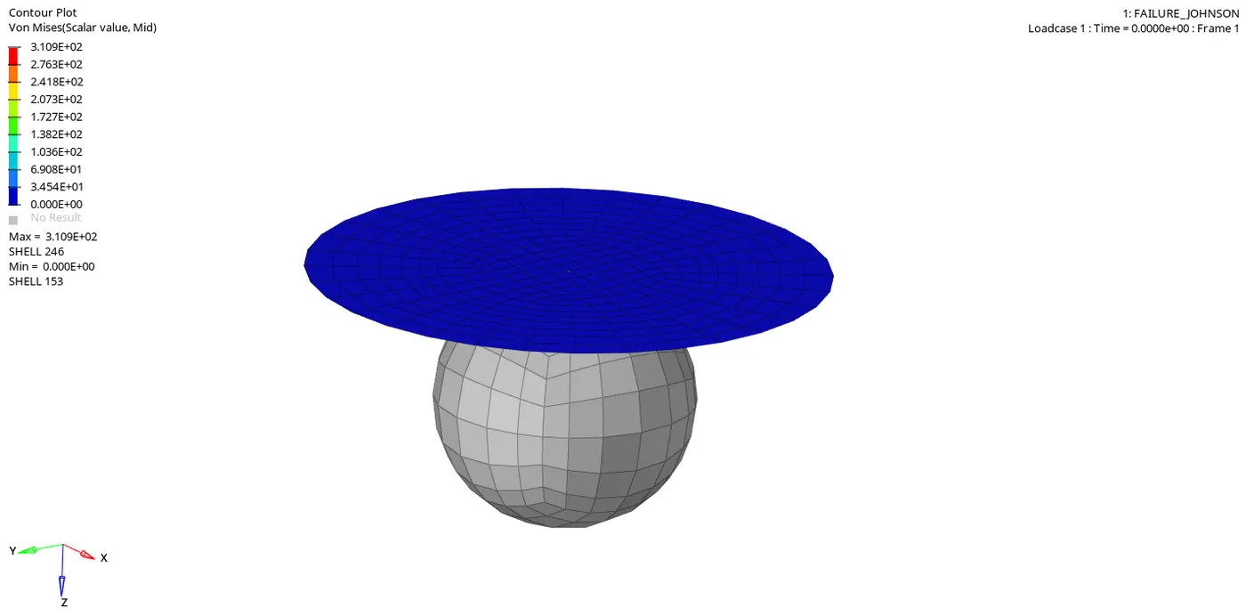
Simulation for Case3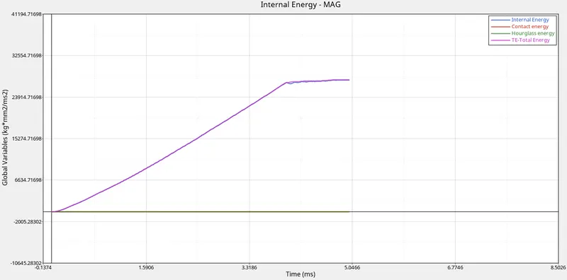
Graph plot for Case3
Case 4: In this case we need to set the value for EPS_p_max as zero and then run the simulation. This value of eps_p_max is called the Plastic strain for tension, compression or shear for the material. This failure is like asombined failure constant for the material.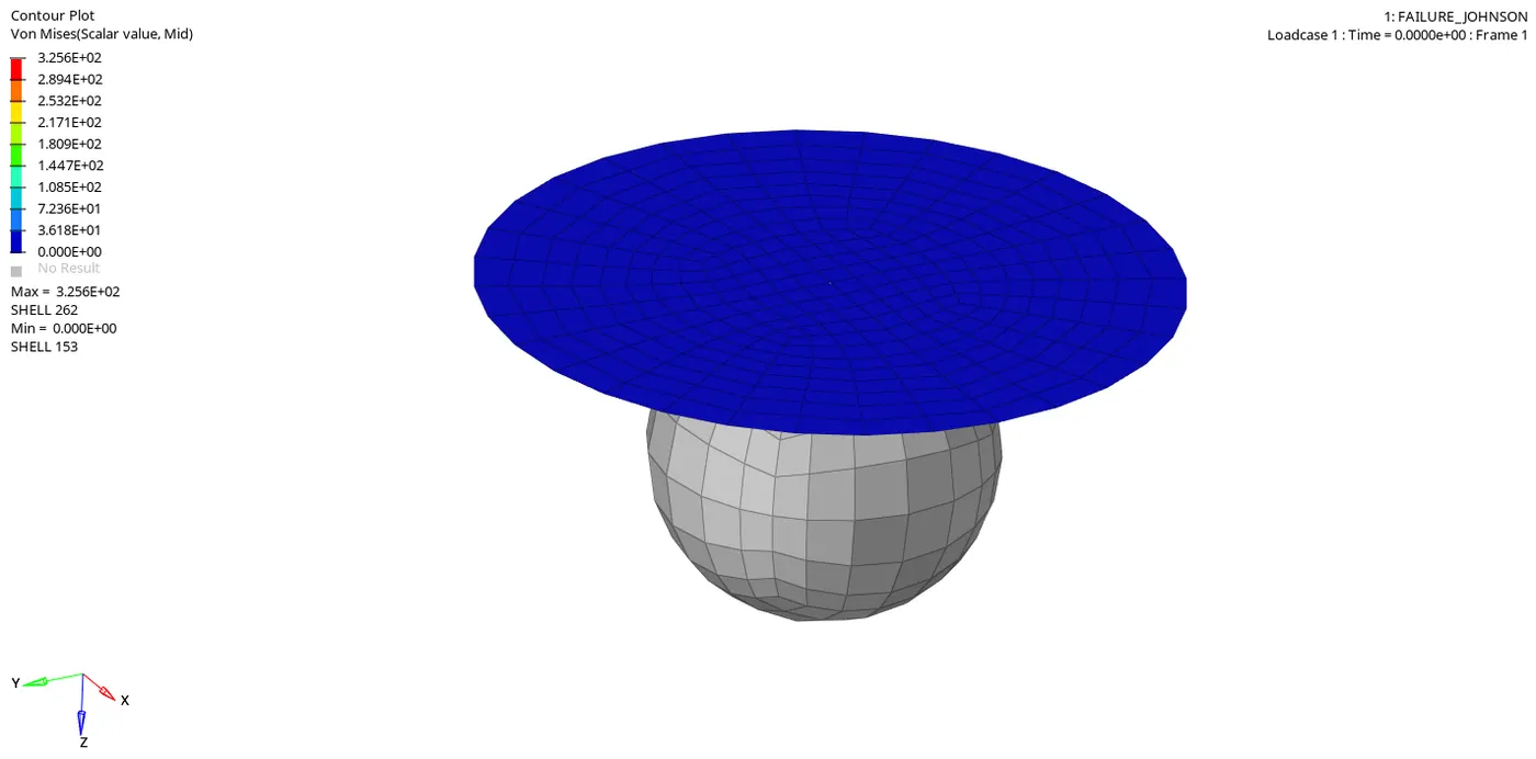
Simulation for Case4
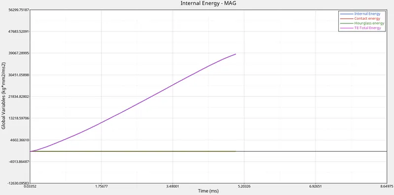
Graph for Case 4
Case 5: In this scenario, we convert the model to Law1. We can use the same material values that we used in the earlier simulations. These values are : Youngs modulus(E) = 71000, `rho` = 0.0028, `mu`= 0.33
We know that the Law1 uses and makes the material behave like a proper Elastic material. So when we use this law, we are basically making the material properly elastic. Because the material is behaving in the elastic properties, the Von missses stresses induced will be a lot larger as seen from the simulation video below: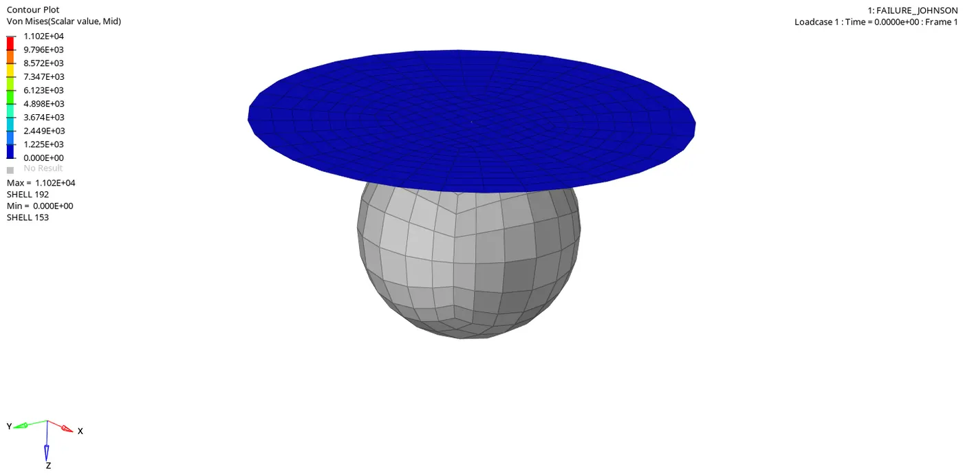
Simulation for Case5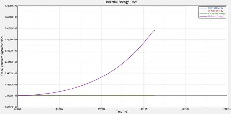
Graph Case5
Case 6: In this case, we need to convert the given model into Law36 which represents the Elasto-plastic properties of a material. We need to define a curve in this case as well for the material properties to be applied. We also have been given the necessary values such as the following:
Eps_p_max: 0.160
Eps_t1: 0.1
Eps_t2: 0.11
To define a curve, we need to right click in the tree and then select the Create option and then further choose the Curve option in it. 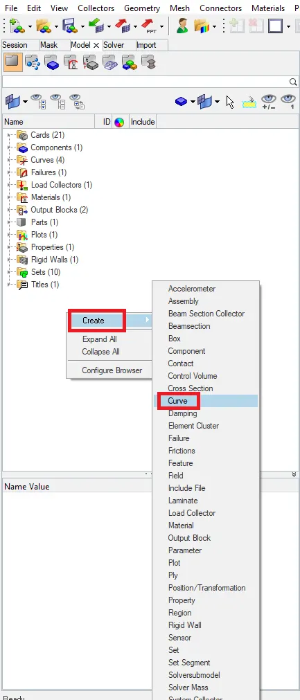
Create -> Curve
After this option was set, we then use the "New" option and set the name of the curve. Then we later give in the values that are to be fed so that we get a proper curve. Then this curve is to be given as an input for the solver while setting the Law36 for the material. This curve will be an input for "N" in the material card. This "N" defines the function on which the material behaves.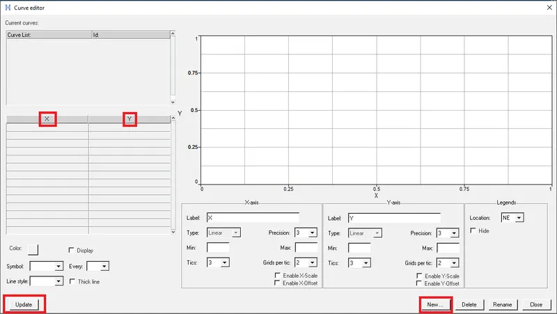
Curve Creation
After all the inputs were given, we then need to run the simulation. It may look as the following: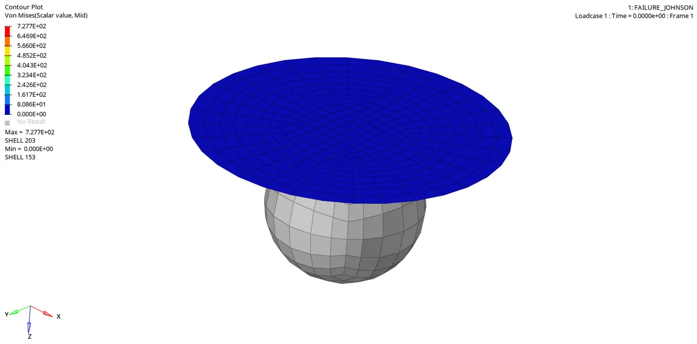
Simulation for Case6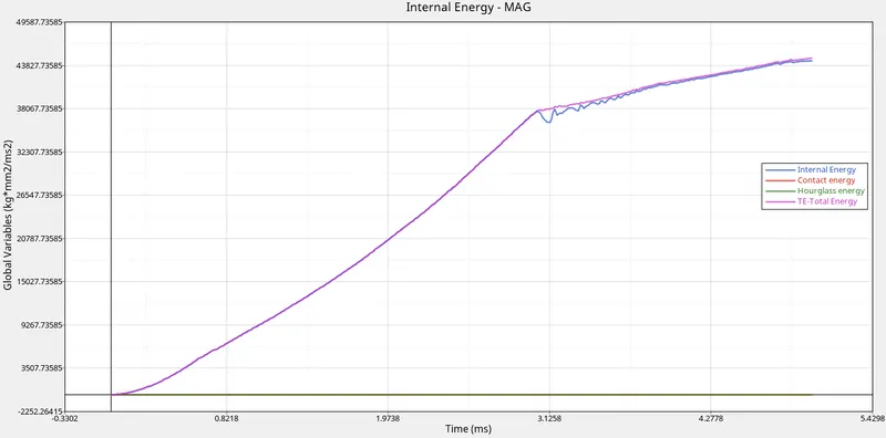
Graph plot Case6
Case 7: In this case, we are to change the Shell properties of elements and run the Base simulation for the material using the Law27 for the material card. We change the Elemental property to the best recommended values, i.e. Ishell = 24, Ismstr = 2, Ish3n = 2, N = 5, Ithick = 1, Iplas = 1.
To change the property of the elements, we need to use the Property card and then change the values as mentioned above. 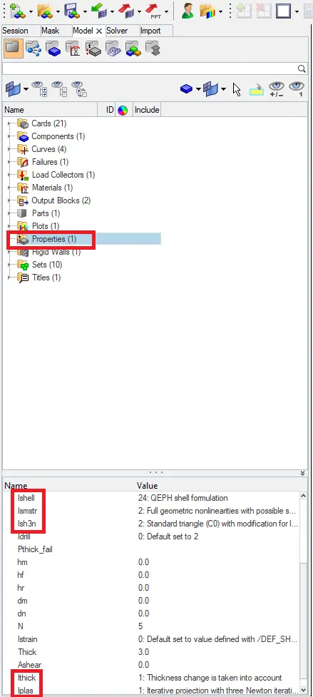
Properties changed
After the properties were changed, we then need to run the simulation as it is. 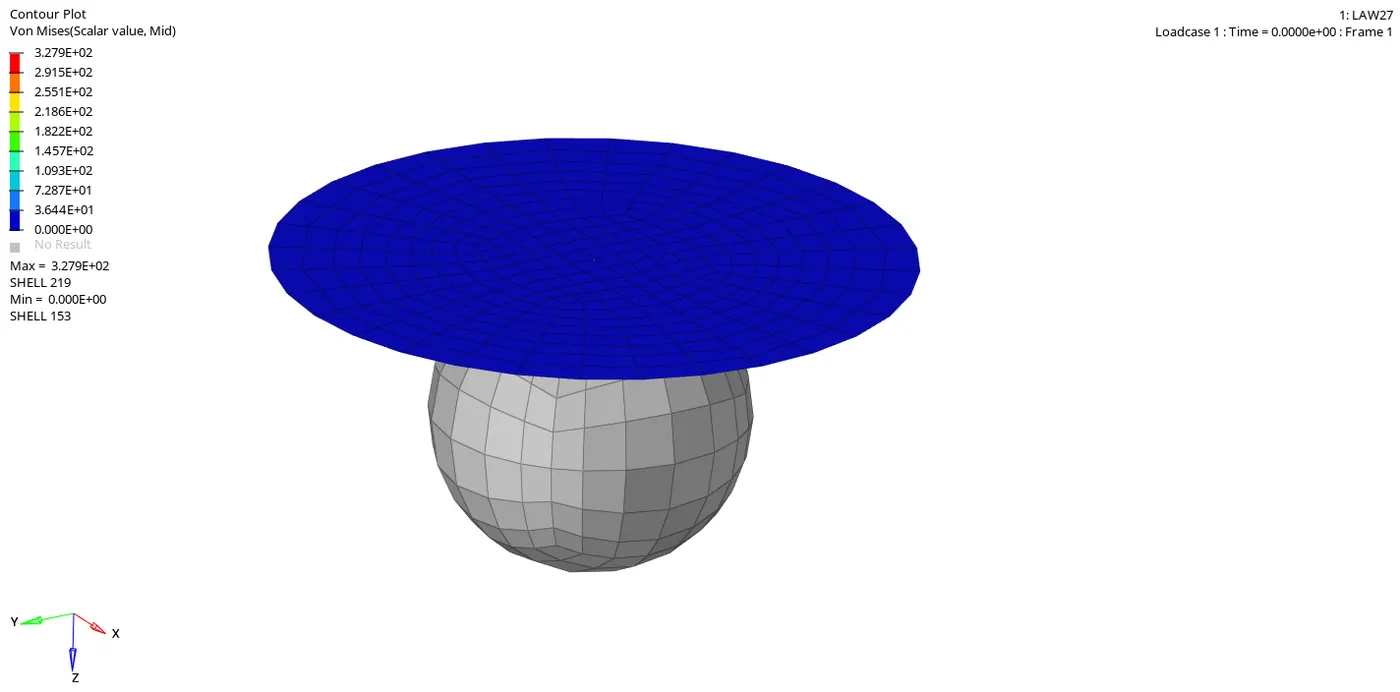
Simulation for Case7 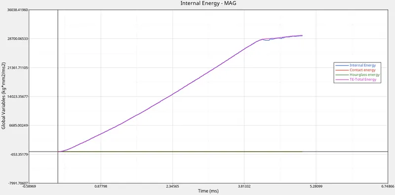
Graph plot Case7
We have seen all the seven cases and their description as well by now. So The next step is to draw certain conclusions from the Simulation and the different graphs we have already plotted. Before we get onto the next step, we should understand the basic term on which the entire comparison is based on. The term in used is called, Von Misses Stress.
Von Misses Stress: It is a criteria that is used to determine if a given material will yeild or fracture. This is used mainly in the cases of Ductile Material.
So, basically, if the Von misses stress `gt`yeild limit, then in that case the material will fail.
Case1 v Case2: In Case 1 we have the Values for Ifail_sh, Dadv, Ixfem different than in Case 2. The overall picture with these values is that they define how the material is supposed to fail after the criteria is crossed. the material can either get deleted or we can even let the cracking on the surface happen as it was supposed to happen on the material.
In both the cases, we have a very comparable Von misses stress (Case1- 316 MPa, Case 2- 295MPa)
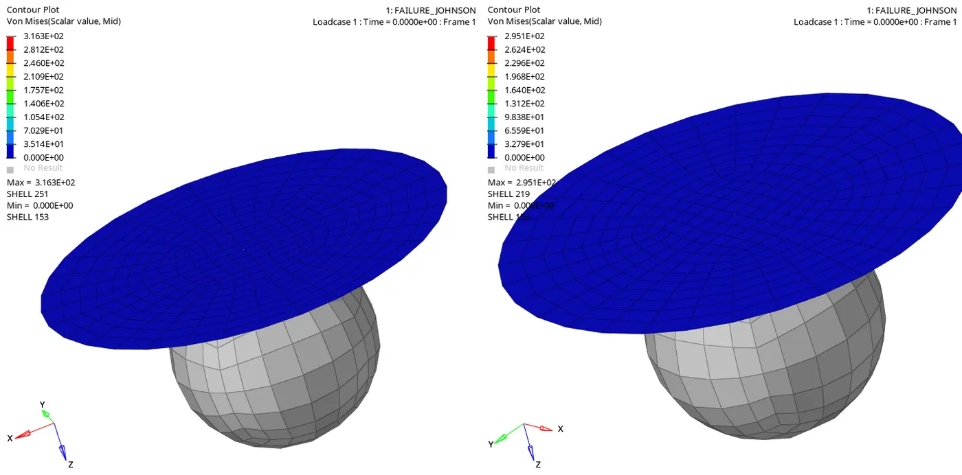
Simulation for Case1 v Case2
From the simulation, we can observe that in case1, the elements break off much more abruptly than in case1. 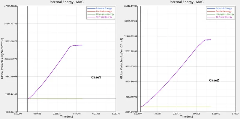
Graph plot for Case1 v Case2
In this case we can see that the Total Energy for case 1 is approximately 27500 mJ and in case 2 it is approximatel 31000mJ. So from these values we can understand that much more energy was absorbed in the case 1 and that deformation is more in that case as well. The values of Internal Energy also point to the same. In case1 the Internal Energy is approximately 27300mJ and in Case 2 it is 31000mJ. Since The value is lesser in Case1, it indicates that the plate broke much before in case1 than in case 2. The hourglass energy is pretty much constant throughout both the simulations, this means that the simulation occured without any hourglass errors occuring in it.
Case3 v Case4:
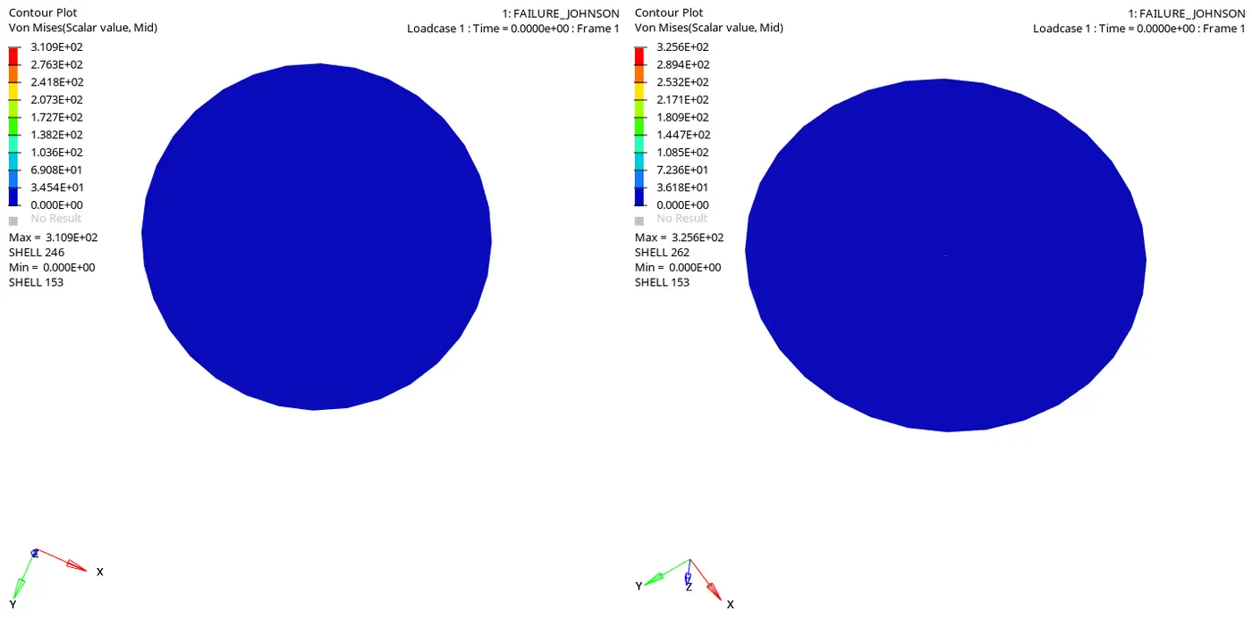
Simulation for Case3 v Case4
We can compare the von misses stress in both the cases here. In case1, the maximum von misses stress reached 310MPa whereas in Case2, the maximum Von misses stress recorded was 325Mpa. From the simulation, we can see that the elements break off much later and that the breakage in the elements is much more uniform, indicating that the elastic properties are much better in case4 than in case3. 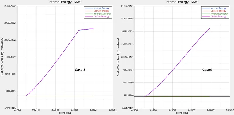
Graph for Case3 v Case4
From the graph plots for Case3, we can see that the Internal Energy Line(Blue line) increases upto a certain value and then almost stabilizes. From this point we can conclude that the elements started breaking off at this point in time. In case4, we can see that Total energy Line(pink line) and the Internal Energy line(blue line) runs parallel to each other and is continuously increasing as well. This means that in the simulation, the Deformation is continuously occuring.
Case5 v Case6 v Case7:
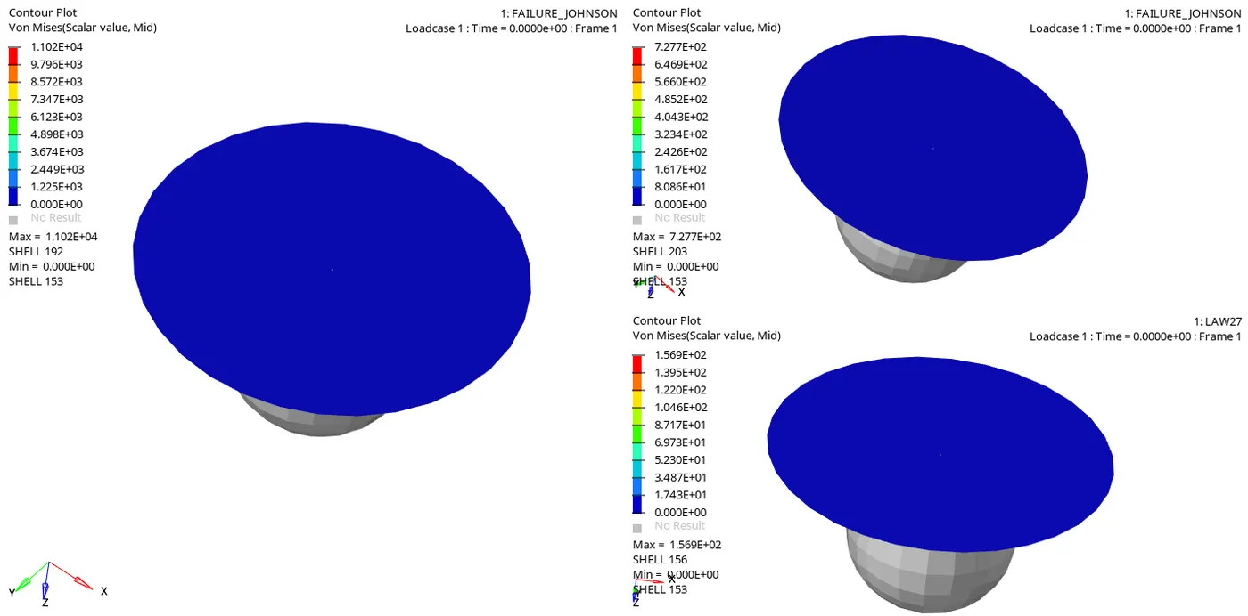
Simulation for Case5 v Case6 v Case7
This is how the simulation is occuring in all the three cases. We can observe that the value of Von misses stress is as follows:
Case5: 1102MPa
Case6: 727MPa
Case7: 327MPa.
In Case5, Since the material property is Purely elastic, we can that there is no breakage of elements and that the plate stretches itself thereby the von misses stress in that case is also the highest amongst all the seven cases.
Also, from the Von misses stresses, we know that the element is most likely to break the earliest in Case7 out of the three. To confirm this, we can see the next photo.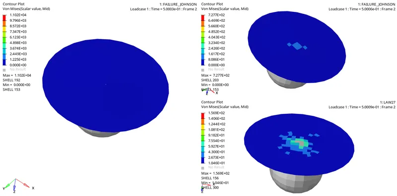
Element Breaking point
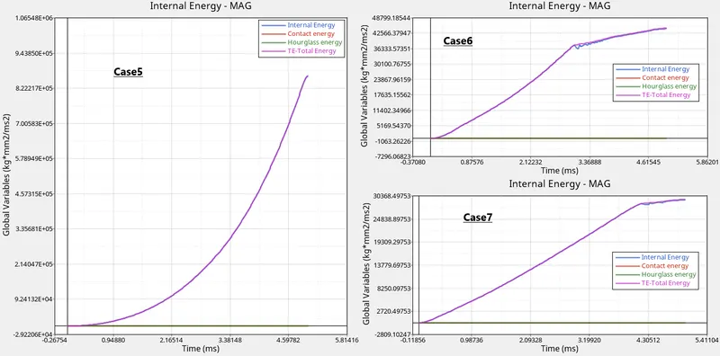
Graph plot for Case5 v Case6 v Case7
In Case5 Graph, we can see that the Total Energy is continuously increasing because of the Elastic properties of the material set. in the Case6 and Case7, we can see that the Total Energy curve(pink line) and the Internal Energy Curve(blue line). We know that Internal Energy in this case can be summarized as the Energy that the energy that the plate can hold. So we can understand the Internal Energy curve will flaten after the plate is broken because the Plate cannot hold any amount of energy after that.
From the Energy plots that we have drawn, we can see that the Hourglass energy has remained constant. This means that the solver has not added any artificial energy to the system because no Hourglass error took place in the system.
To summarize the energy error and all the other important characteristics of all the seven cases, the following table was made:
| Case number | Total number of cycles | Energy Error | Mass Error | Total Simulation Time. (s) |
| 1 | 49380 | -0.8% to 1.3% | 0.00% | 106.71 |
| 2 | 49217 | -1.1% to 5.9% | 0.00% | 113.51 |
| 3 | 49408 | -0.6% to 1.2% | 0.00% | 104.72 |
| 4 | 49304 | -0.6% to 1.2% | 0.00% | 103.14 |
| 5 | 47969 | -0.6% to 4.0% | 0.00% | 100.41 |
| 6 | 52201 | -0.9% to 0.7% | 0.00% | 111.25 |
| 7 | 49508 | -0.6% to 1.1% | 0.00% | 106.63 |
Table for all the Seven Cases.
- Conclusion: In conclusion I would like to state that this assignment helped me understand how the material and elemental properties affect a simulation.