Assignment 3-2D Element Formulation Challenge

ASSIGNMENT - 3

Overall objective:

The main objective in Assignment 3 is to run the simulation with & without change in element properties and plot the energy graphs using Hypergraph in both the cases and comparing both results by using graphs that what will be change between both cases.

CASE - 1

Objective:

The main aim in case 1 is to import a .rad file and changing run time , no. of animation steps but keeping all the element properties like Ishell , Ismstrn... same and running the simulation & plotting graphs with energy deviations by using Hypergraph.

Procedure:

• File - Import - Solver Deck - Select file from downloaded files location - Import
• Press 'F' to Fit the model on the screen
• Go to Cards - ENG_RUN - change the Tstop value to 55ms as mentioned Run time = 55ms in the question

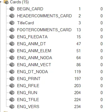
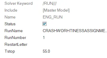
• Than to change number of Animation steps minimum of 25 to max. of 60 as given -
• Start calculating Tfreq as in these we need to update No. of anim steps by

Tfreq = Run time/Number of animation steps

As given above use the value between 25 to 60,

Take, No. of anim steps = 40

Run time or Tstop = 55 ms

Tfreq = 55/40 = 1.375

*Tfreq = 1.375

• Now update the above Tfreq value in ENG_ANIM_DT Card as -

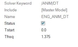
• After updating ENG_RUN & ENG_ANIM_DT cards save the model once in the required file location by going to -
• File - Save/Save as - Location in the disk - Mention the File name - Save - While saving this File try to create a New folder as there will be so many working files stored in that
• Now go to Analysis panel - Radioss - Mention input file path - in the options use '-nt 4' - than hit Radioss for simulation -

• After clicking the radioss the simulation will run and we will get the dialog box open that contains all the values as -

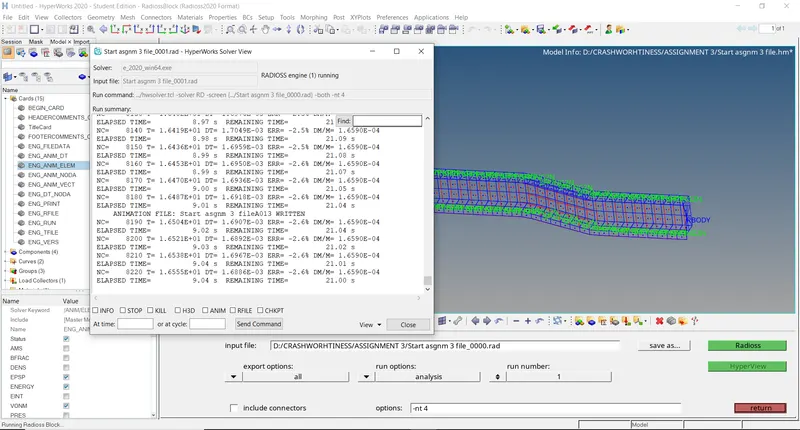
• Now again by going to the stored location check the values using any text editor like notepad or wordpad it will look like this -

• From this file check for % Energy errors and mass error:
• Mass error:

It is nothing but extra amount of mass added to meet specified Timestep , here it has a non zero value i.e.. it must be added near the node. Mass error should also be not more than 0.05 or 5%

• Energy error:

Energy errors mainly indicates energy added or Dissipated , here as the value in negative means the energy is dissipated but in this case it doesnt matter much because as it is of fully integrated elements due to which we can leave that but if the value is positive i.e.. above +10% those should be considered it should be considered and there is another method for that.

• As from this we can say that % Energy errors should be in negative values and if at all it is positive value it should contain only till +5% only
• But coming to this model it has no Energy errors and also mass error is also considerable as value of that is also constant i.e it passes both conditions and now we can start plotting graphs using Hypergraph
• After this go to Hypergraphs select the file name which contains series .T0.. as like this

• Now start selecting with which variables it should be plotted as
• In X Type mention Time than - Global variables - Internal energy - MAG - click on Apply - By this we get curve showing Internal energy with Time and the graphical window looks alike this -

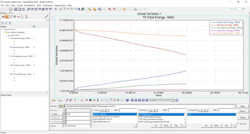
• Like above start Selecting Energies which should be plotted by same method
• These graphs are plotted after doing all the calculations but without involving manual interference by software itself but if we want to check that it can be calculated as below:

Kinetic energy 'kE' = 1/2 *m*v2

where, m - mass in grams

v - Velocity in m/sec

• To check the mass Go to Tools - Mass details - Mass only the dialogue box will be opened containing masses as -

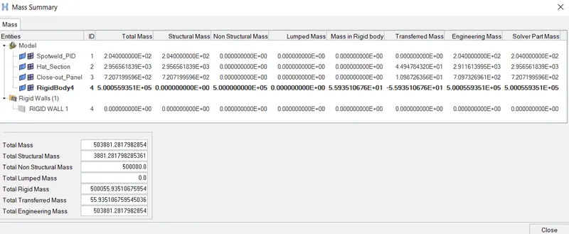
From this, we get to know that mass 'm'= 503881.29 gms

• After this to check the values of velocity Go to View - Browsers - Hypermesh - Solver - After clicking on solver we will get cards in the left side of hypermesh GUI from there -
• Select - INVEL - again INVEL - Initial velocity - after clicking on this we will get a dropdown which has velocity values as below -
  
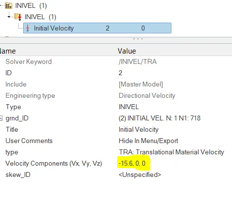
• By this we get Velocity 'v' = 15.6 m/sec
• Now these values to be substituted in the above KE formula so that we will get a final value which will be Autocalculated by computer software and Kinetic energy graph will be plotted according to the value this can be manually calculated as mentioned above.
• Internal energy will be calculated as follows:

*IE = Q +or- W

where,

Q = Heat transfer coefficient in W/KW

W = Work in J/KJ

• Total energy = Internal energy+ Kinetic Energy + Contact energy + Hourglass energy

  * TE = IE+KE+CE+HE

• Time - Global variables - KE , Constant energy , Hourglass energy , Total energy - Click on apply for each energy the graph will be plotted with the values and after plotting with all the energies it will be -

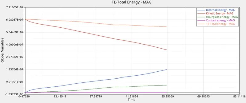
• The energies are shown with colours that is one colour with one energy
• Now for plotting Rigid wall forces again start with new plot in File as -
• File - New - New plot - by this it will clear old graph and starts with new
• After creating new plot - select Time in X type and - Near Y type select Rigid wall forces (R wall forces) - Select on which axis the values to be shown as Fxx , Fyy , Ftangent (Frictional force) , Fresultant etc... and for this whole graph window looks as -

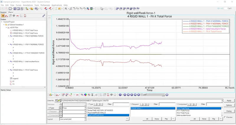
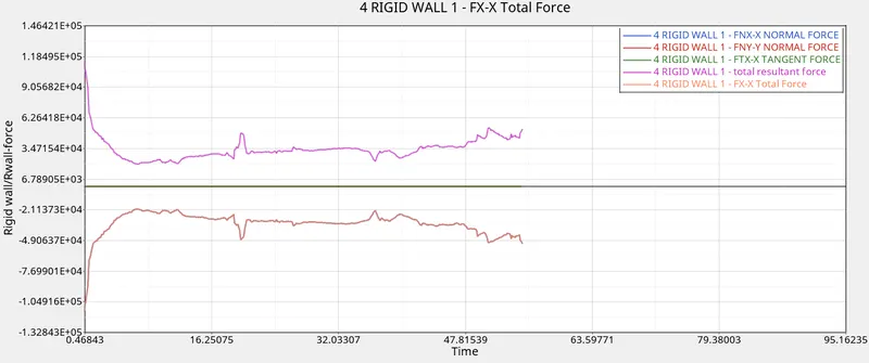
• In this Picture it shows only graphical area with Rigid wall forces in closer view-

Result:

By performing all this operations , according to the question there will be Energy graphs & Rigid wall forces given will be plotted in Hypergraph by changing only Run time and Number of animation steps in Hypermesh file of model and with this values the graphs will be created.

CASE - 2

Objective:

The main aim in case 2 is to import a .rad file and changing all the element properties like Ishell , Ismstrn... and running the simulation & plotting graphs with energy deviations and R wall forces by using Hypergraph.

Procedure:

• File - Import - Solver Deck - Select file from downloaded files location - Import
• Press 'F' to Fit the model on the screen
• Go to Cards - ENG_RUN - change the Tstop value to 55ms as mentioned Run time = 55ms in the question

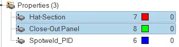
• Than Go to Properties - Select the first two mentioned properties and there will be a dropdown opened there it should updated as given values in the question -

Recommended properties in question file:

Parameters		Comment
Ishell =24		QEPH 4 nodes shells are best combination of cost and accuracy.
Ismstr=2		Full geometric nonlinearities (default)with possible small strain formulation activation in RADIOSS Engine.
Ish3n=2		Standard 3 noded shell (C0)with modification for large rotation(default)
N=5		Number of integration points set to 5 for accuracy bending.
Ithick=1		Thickness change is taken into account for accuracy.
Iplas=1		Iterative plasticity for good accuracy.

• Update all these values in the dropdown of first two properties as Ishell = 24, Ismstrn = 2, I sh3n = 2, N=5 , Ithick = 1 , Iplas= 1

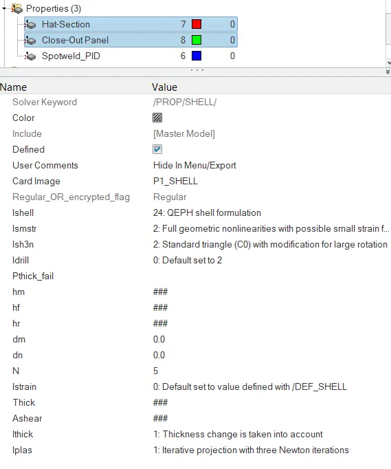
• Here each value has its own significance :

Ishell = 24:

- This is an improved under-integrated 4 node element with 1 integration point on the surface with physical hourglass stabilization

- This is the best compromise between cost & quality

Ismstr = 2:

- This is used for problems with large displacements & strains

- Strain computed based on the current element shape with the derivate of the shape function

Ish3n =2:

- This is used as Standard triangle(CO) with modification for large rotation with 1 integration point on the surface.

- No Hourglass deformation with Low CPU cost

N = 5:

- This are number of integration points which is recommended for good & accurate calculations

Ithick =1:

- Here thickness change is taken into account

Iplas = 1:

- This Iterative projection with Newtons method which is more accurate and mainly used incase of Plastic surfaces.

• After updating these values save the model once
• Than again start simulation for this also by -
• going to Analysis panel - Radioss - Mention input file path - in the options use '-nt 4' - than hit Radioss for simulation -

• After clicking the radioss the simulation will run and we will get the dialog box open that contains all the values as -

• Now again by going to the stored location check the values using any text editor like notepad or wordpad it will look like this -

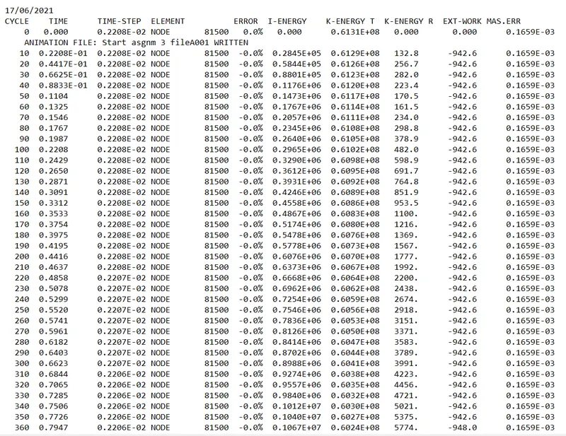
• Mass error:

• It is nothing but extra amount of mass added to meet specified Timestep , here it has a non zero value i.e.. it must be added near the node. Mass error should also be not more than 0.05 or 5%

• Energy error:

• Energy errors mainly indicates energy added or Dissipated , here as the value in negative means the energy is dissipated but in this case it doesnt matter much because as it is of fully integrated elements due to which we can leave that but if the value is positive i.e.. above +10% those should be considered it should be considered and there is another method for that.

• Here also there is no problem with % Energy error values and also mass error now we can proceed to crete graphs using Hypergraphs

• After this go to Hypergraphs select the file name which contains series .T0.. as like this

• Now start selecting with which variables it should be plotted as
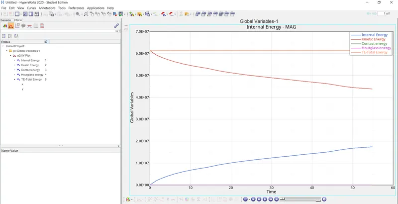
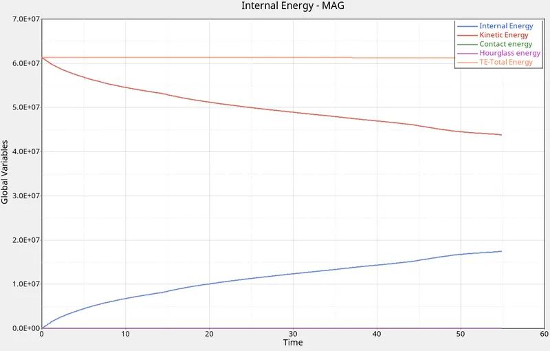
• In X Type mention Time than - Global variables - Internal energy - MAG - click on Apply - By this we get curve showing Internal energy with Time .
• By using the data which we loaded in the hypermesh file the energy and other graphs are created like this

• Now start creating Rigid wall forces by using Hypergraphs by going to -
• File - New - New plot - by this it will clear old graph and starts with new
• After creating new plot - select Time in X type and - Near Y type select Rigid wall forces (R wall forces) - Select on which axis the values to be shown as Fxx , Fyy , Ftangent (Frictional force) , Fresultant etc... and for this whole graph window looks as -

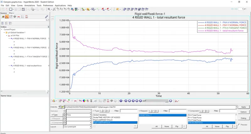
• The closer view of Rigid wall forces after updating Element properties -

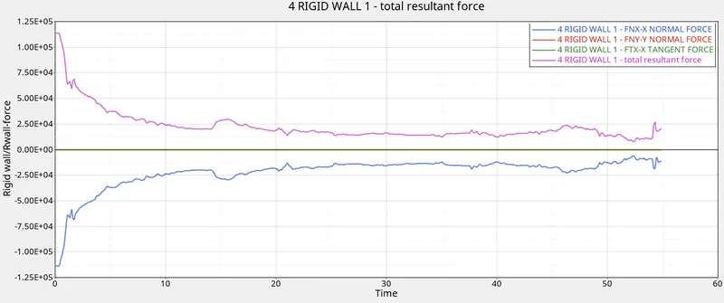
Conclusion:

Finally by going through this procedure we will get the simulation which has energy & mass error where element properties are also changed and by using same file in Hypergraph we get graphs with all type of Energies and Rigid wall forces and clearly shows how these values are changing and when are they changing can be clearly known.

DIFFERENCE BETWEEN CASE 1 SIMULATION AND CASE 2:

Here the main differences for each and individual property/type will be discussed-

1. Run time & No. of Animation steps:

-The main thing here is that the Run time & No. of animation steps will be similar in both the cases i.e...

*Run time = 55ms

*No. of Animation steps = 40

2. Energy error & Mass error:

-Here by coming to this errors both are almost similar as -

*masss error = 0.1659E-3

*Energy error = -0.0% .....

-But the only thing changing is Timestep value as in the Case 2

Timestep values for,

Case 2 = 0.2208E-01

but for Case 1 it is around 0.2240E-01

-So by this we can clearly state that Timestep for Case 2 i.e.. after applying Element properties is lesser than that of case1

3. Internal Energy:

- IE is calculated as :

IE = Q +or- W

where,

Q = Heat transfer coefficient in W/KW

W = Work in J/KJ

But here,

Q = 0

so, IE = W

= Force * Displacement

Where, F = mass * acceleration =m*a

Finally we get , IE = ma*S

- This calculations can be used to crossverify already software created energy graphs

- But here comparing both the cases initially the internal energy is Null but after a certain time period the graph gradually increases , practically it can be said that before crash the workdone is zero but suddenly after the crash the graph starts going upwards.

- In case till half of the time the graph is increasing in normal curve but after that it is indicating a sudden increase in IE

- But in Case 2 from starting to ending it is slowly and gradually increasing

4. Kinetic Energy:

- KE is calculated as below,

Kinetic energy 'kE' = 1/2 *m*v2

where, m - mass in grams

V - Velocity in m/sec

- KE initially is very high due to high motion but suddenly starts decreasing after hitting a sudden obstacle both cases shows same thing but,

- In case 1 it is indicating decrease in KE very fastly and rapidly

- But in case 2 there is slow and gradual decrease in KE curve

5. Contact Energy:

- Contact energy in both cases is same which is attached to the X -axis line as this energy is always formed near the contact surfaces only.

6. Hourglass Energy:

- Hourglass is a type of deformation occurs near the nodes as it will start changing its shape & size suddenly

- This is formed because of,

DT < T

i.e.. The actual time taken to reach from one node to another is less than the time taken to reach more distance by this forces and stresses in some cases

Than it starts deformation in the element as due to artificial energy it has reached early by this we will face deformation near elements

- Hourglass energy is also called as 'Artificial energy'

- Here calculation of stress will be from node to node i.e..

- Near each node there will be a seperate velocity , seperate acceleration and seperate stress which are linked one to the other

velocity = Acceleration/time

Displacement = Velocity/time

Strain 'e' = dL/L

Stress = E*e or PL/AE

Like this we can calculate one after the other by substituting the values,

Always *DT > T as to overcome with this Hourglass energy

7. Total Energy:

- Total energy can be calculated as :

Total energy = Internal energy+ Kinetic Energy + Contact energy + Hourglass energy

* TE = IE+KE+CE+HE

CHANGES MADE FOR	CASE 1	CASE 2
Run time	Yes	Yes
No. of Anim steps	Yes	Yes
Element properties	No	Yes
%Energy error	-	-
Mass error	-	-
Internal energy	Yes	Yes
Hourglass energy	Yes	Yes
Contact energy	Yes	Yes
Total energy	Yes	Yes
Rigid wall forces	Yes	Yes
Radioss Simulations	Yes	Yes