Assignment 3-2D Element Formulation Challenge

OBJECTIVE :

Comparison of results with base simulation and improved shell element properties

1.Using the crash beam file provided, change the run time to 55 ms.

2. Change the number of animation steps during simulation to a minimum of 25 and maximum of 60.

3. Run the base simulation without any modification to element properties.

4. At the end of the simulation, do the energy error and mass error checks and determine whether results would be acceptable.

5. If acceptable, Plot rigid wall forces, internal energy, hourglass energy, contact energy, total energy of the simulations.

6. Change all the shell elements properties to recommended properties, save this as separate, rad files and run the simulation.

7. Follow steps 5 and 6.

8. Create a brief report comparing all the results from steps 5 and 6 for both simulations.

9. Comment whether there is any change in the results and why there is any change in the result.


PROCEDURE :

1. Import the given crash beam file to the Hypermesh window. And change the view to shaded elements to see the meshed component clearly.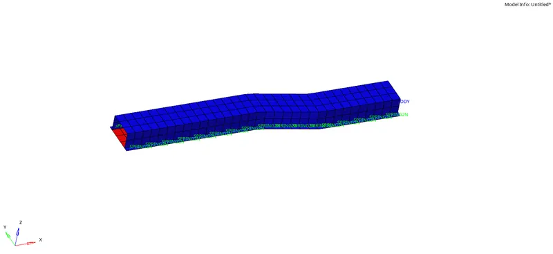



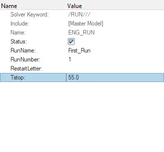
2. Now, to change the run time to 55ms, go to Cards Collector >> ENG_RUN >> Tstop >> change to desired value ( here the given default value was 60.0 ). It has been changed to 55ms from 60ms

       
                                              
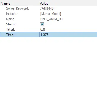
3. Now, the number of animation steps during has to be set between min.25 to max.60. We select the value of 40 animation steps. Now, to set this 40 animation steps, the Tfreq value has to be changed.

Tfreq = ( Total run time / no. of. animation steps required ) 

So, Tfreq = (55/40) = 1.375

Now, to set the Tfreq value, go to ENG_ANIM_DT >> Tfreq >> Set the desired value (Given default was 1.0, It was changed to 1.375)

                                                

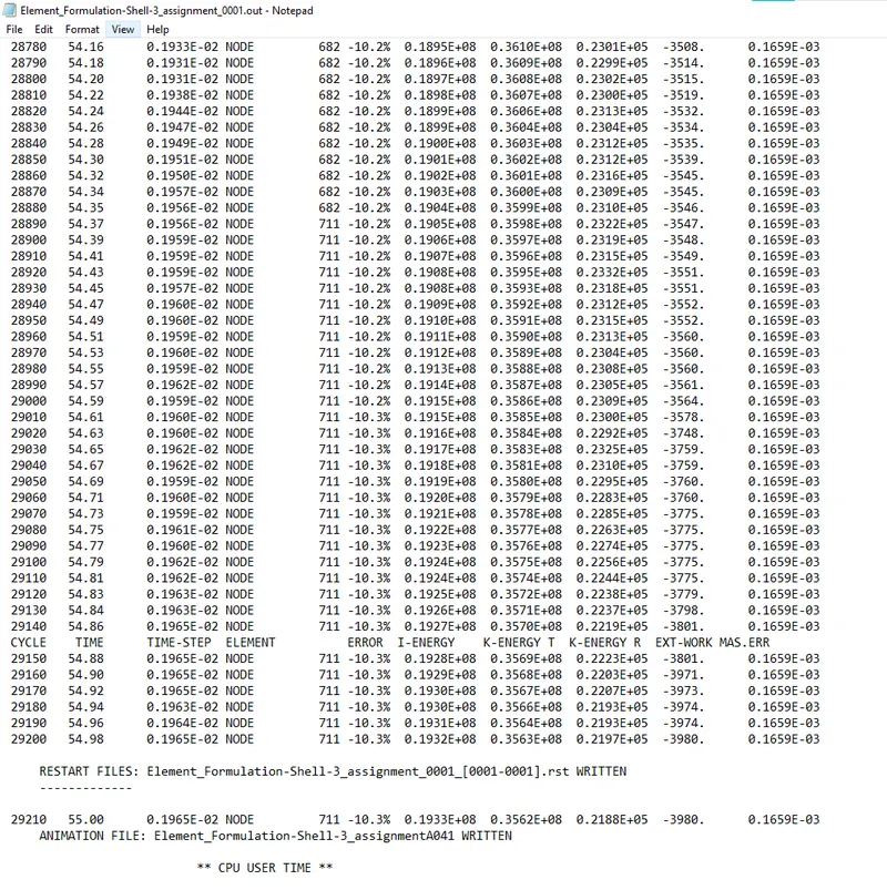
4. With the Tstop, Tfreq and animation steps set, we can now export the corresponding file to the radioss solver and proceed with the analysis to check the energy error and mass error. Make sure to enter the ( -nt 4 ) In the options tab ( to access number of cores in the hardware which is hardware specific )

        

Now, while checking the results, we can observe that the energy error starts from -0.0% and goes upto -10.3% and the Mass error remains the same 1.65490E-4 throughout the simulation which is within the range of acceptance.

                          

5. Now, we can proceed with Ploting rigid wall forces, Internal energy, Hourglass energy, Contact energy and total energy of the simulation.
For this, we need to export the output file and view them in the Hyperview and Hypergraph windows to see the animation and the energy plots.


To Open the animation file, we need to search for .h3d file and open it in the Hyperview tab to view the animation. Once it is opened we can see the Contour  Options to View the various phenomenon, Here we need to check the Displacment and the Hourglass energy. 
Firstly the Hour glass energy is observed. 

                           

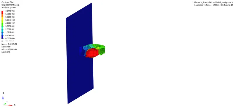
From the above image we can see that the maximum displacement was about 761mm 

6. Now, let's see the Hourglass energy of this crash tube. By changing the viewing option from displacement to Hourglass we can see the Hourglass energy generated in this crashing.

               


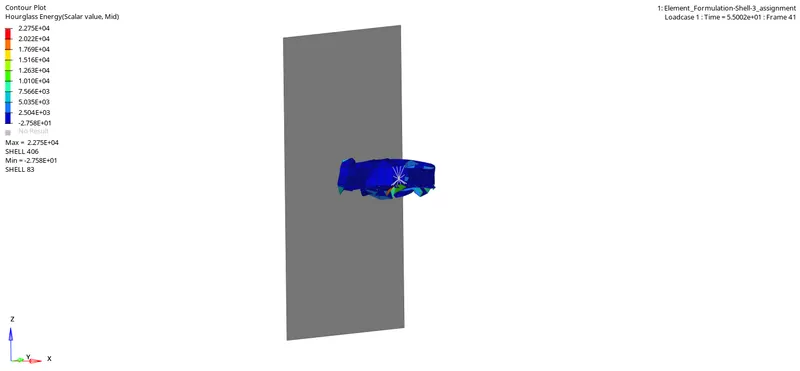
7. Now, to see the Global Variables, we can split the window and open up Hypergraph in the other window. Here we need to import the T01 ( Time History File ) to view all the global variables like Hourglass energy, internal energy etc.

Once the File is imported, Fix time along X axis and set the global variables Internal energy, kinetic energy, etc in the Y axis and observe the results :

                         

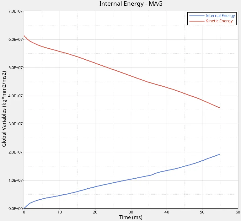
We can see that the Kinetic Energy is maximum at the starting since a huge force is applied to the crash tube which possess certain mass and then it gradually decreases since the component deforms.
Similarly, we can see that the Internal energy is minimum while starting and it gradually increases as the component starts to deform and absorb the energy.

8. Now, let's see what the Rigidwall forces are and the Hourglass energy plots :

                         

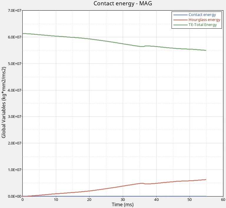
Since the elements used were of reduced integration, there are hour glass energy which increases from the starting.|
The Total energy also slightly decreases from the beginning and this is due to the energy error and the hour glass energy produced.

9. Let's check the Rigidwall Resultant forces :

                          
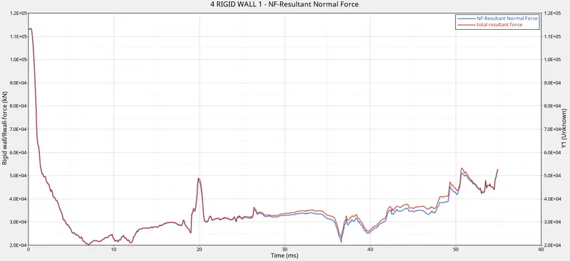
We can see that the Total Resultant Force is in a non linear manner which is slightly above the resultant normal force. There are certain spikes in between which indicates there occurs certain spike in force which is hitting the rigidwall.


Now, Let's see what the results are when we change the Properties of the elements as recommended and check the results. 
Here are the changes made to the Properties:

Parameters		Comment
Ishell =24		QEPH 4 nodes shells are best combination of cost and accuracy.
Ismstr=2		Full geometric nonlinearities (default)with possible small strain formulation activation in RADIOSS Engine.
Ish3n=2		Standard 3 noded shell (C0)with modification for large rotation(default)
N=5		Number of integration points set to 5 for accuracy bending.
Ithick=1		Thickness change is taken into account for accuracy.
Iplas=1		Iterative plasticity for good accuracy.

Once all these were changed, and the Tstop set to 55ms and the Tfreq set to 1.375 ( for 40 animation steps ) now let's run the solver and check the mass and energy error.

                        
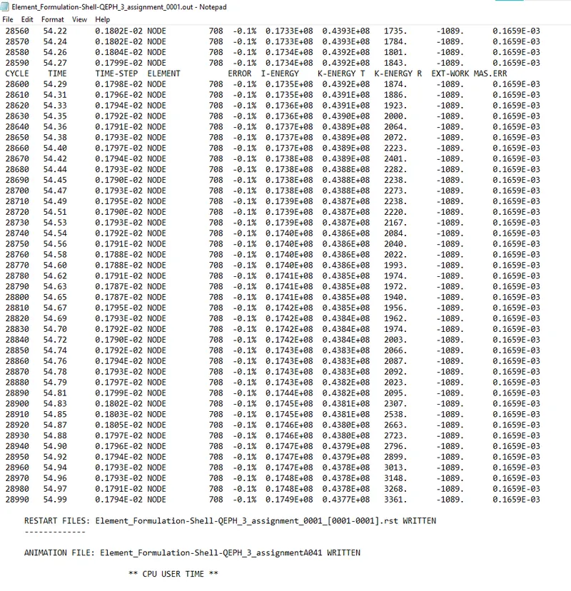
Here we can see that the Energy error is -0.1% which is a great sign and the mass is almost the same 0.1659E-03. So, this is a well accepted result. Further we can proceed with the contour plots and the global variables plot and cross check the results with the previous condition.

To check the Contour plots and animation, Open the .h3d file in the Hyperview and switch to contour option. Let's see the displacement created in the simulation.

                       

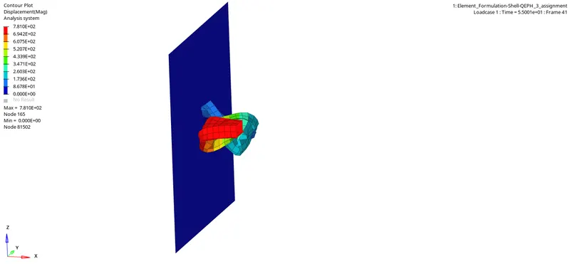
We can see that the maximum displacement is found to be 781mm.

Now, switch the contour to Hourglass and check the hourglass energy created in the crashing tube.

                         

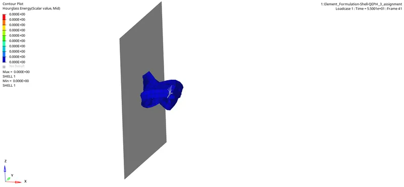
The Hourglass energy seems to be non existant in this condition.

Now, Open the T01 ( time history file ) of this phenomena in the Hypergraph where the element properties were changed to check the Global variables and the Resultant forces. 

After Opening the T01 file, Fix Time along x-axis and Fix the global variables Internal energy, Kinetic energy, Hourglass energy and Total energy along y-axis and plot the graph.

                        

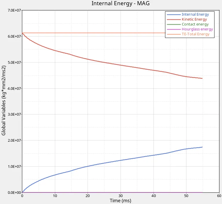
We can clearly see that there is no Hour glass energy, Kinetic energy falls and the Internal Energy gains throughout the time period. The Total Energy seems to be consistent throughout the Crashing.

Now, create a new plot for time and Rigidwall forces in the same manner.

                          
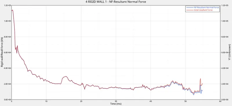
We can see that the Total Resultant force is slightly above the Normal Resultant force and it is behaving in non linear manner.

Since, we have the results on both the element properties, we can see the difference in the results and here are the Evident changes in the result and its possible reason for the changes:

1. TOTAL ENERGY : It is evident that the Total energy is consistent in the second case whereas in the default property the Total energy was decreasing. This is due to the fact that the Energy error changed from -10.3% to -0.1% when the element properties were changed.

2. HOUR GLASS ENERGY : The Hourglass energy doesn't exist in the second case whereas the default element has some hour glass energy. This is due to the type of integration wherein the default follows reduced integration method while in the other case it is Improved Reduced Integration wherein It has the capacity of adding artificial stiffness directly to the material to avoid the Hour glass energy.

3. CONTACT ENERGY :  It is almost the same in both the cases.

4. INTERNAL ENERGY : The Internal energy also increases throughout the simulation in both the cases.

5. RIGID WALL FORCES : The Resultant rgidwall force was dropped in the second case than the resultant force in the default element property.

6. DISPLACEMENT : There is a slight increase in maximum displacement of elements in the second case which is roughly about 20mm when compared to the default property elements. This might be due to the better integration method followed in the recommended element property.


RESULT :

Thus, the simulation has been carried out with both the default element property and with recommended element property and its results like global variables, rigid wall force, hourglass energy, energy errors were compared.


NOTE : The recommended property of QEPH elements has to be applied to both Hat-section & Close-out panel and it is not applicable for the seam weld.