Assignment 3-2D Element Formulation Challenge

Simulation of a Rail Component:

• The objective of the challenge is to run the simulation for the 2 different cases using radioss, then to compare with in them and conclude which is very accurate to the standards.
• Opting the user profile as "Radioss".
• Importing the 0000.rad deck file and the 0001.rad file using the import Solver Deck.

                                                                           

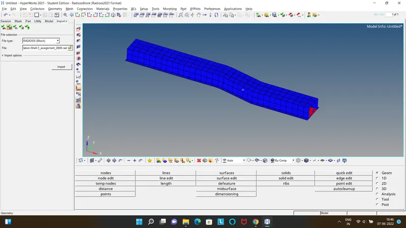
1. Changing the run time to 55 ms.

                                                                                                                             

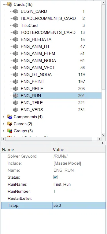
2. Change the number of animation steps during simulation to a minimum of 50 units, ie..., "Animation Time Frequency"=Run Time/Animation Steps=55/50=1.1 and the Tsacle to 0.9 and Tmin to 0.55 as shown.

                                                                              

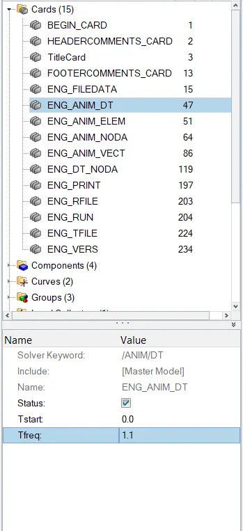
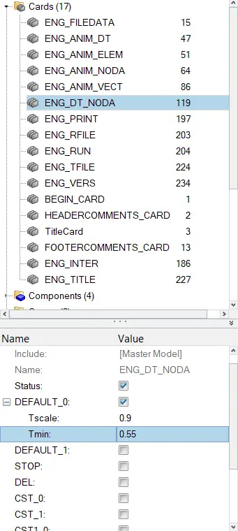
• Export the updated Radioss Solver Deck File and Save it as "Case 1"
• Start a New Hm Radioss File and Import the Case 01 0000.rad File.

3. Running the base simulation without any modification to element properties.

• Analysis>Radioss>Check In the Include Connectors>"-nt 4" in Options>Radioss.

                                                                           

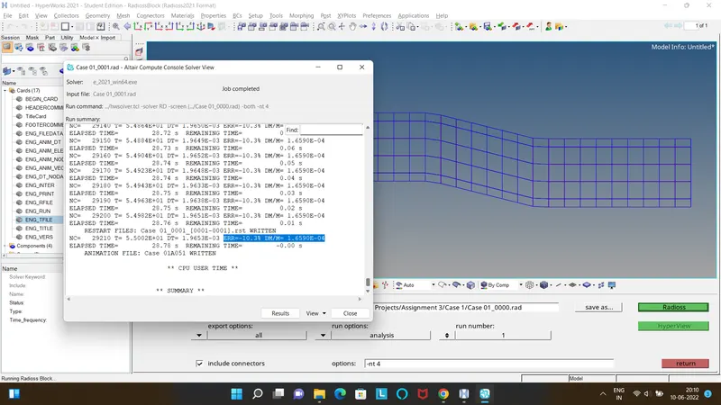
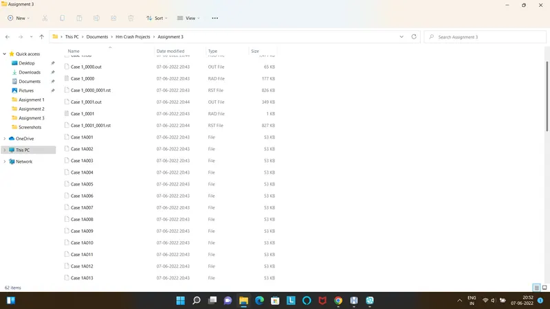
• Go to retrun, If you check the folder where the Case 01 0000.rad file was saved, in the same location with the same case 1 name many file are been created as shown.

                                                                         

• 4.For the above values, Open the Case 1_0001out file(engine output file), scroll down to the bottom at the last cycle ie..., to the 29210 cycle you will observe the 

        Mass Error=0.1659E-04 & Energy Error=-10.3% both the values are Acceptable because the range of the Mass Error & Energy Error is only acceptable when the Mass Error ranges from 0 to 2% and the Energy Error ranges from -20% to 0 

5.Now update the Recommended properties in the properties as shown to the Hat as well as to the close out panel.

                                                                                         

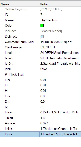
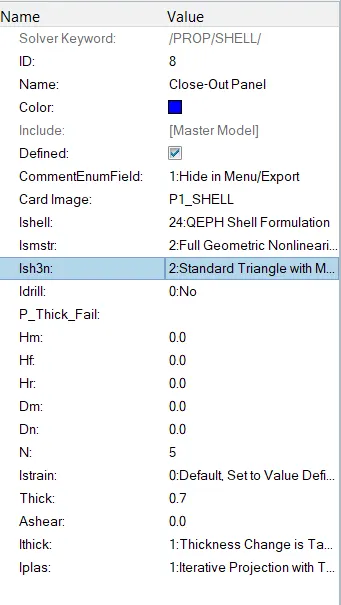
•  export the file again naming case 02 to the different location to avoid the confusion.
• Again open a new model and Import the file to run the radioos as perform initially.
• Files are created similarly.

                                                           

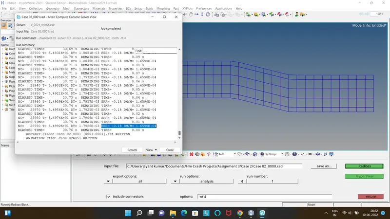
• As per the Case 02 output file, Here the Energy Error=-0.1% & Mass Error=0.1659E-04 and as discussed comparing the Energy Error in both the cases here we can observe that very less Error is occuring, Hence the Case 02 file is more Accurate and Acceptable under Comparision.

                                                             

5.

Rigid Wall Resultant Force:

• Now change the mode from Hypermesh to HyperGraph 2D.

                                                           

• Import the Case 01T01 file.
• Select the Rigid wall forces and total Resultant force in the Drop downs.

            

• On clicking Apply we get a same Display asking units so Set the units to g, mm, ms and hit Apply.

                                                                          

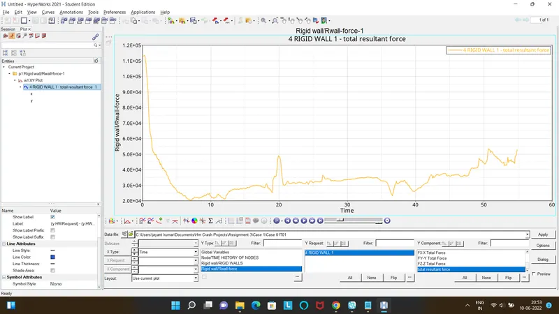
• W.r.t to the given inputs we get a Max value and min value of Resultant forces as shown.

                                                                                                                       

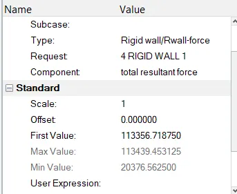
.Hence Max Resultant Force was noticed as 113356.718750 N and the Min Resultant Force as 20376.562500 N.

• Repeating the same importing the case 02T01 file, the Max Resultant Force is noticed as 114153.796875 N. & Min Resultant Force as 7655.160645 N.

                                                                                                                              

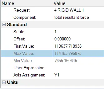
• Comparing both the rigid wall Resultant Force we get the Max force and the min Force w.r.t the Case 02 which is noticed as 114153.796875 N. & Min Resultant Force as 7655.160645 N.

• As the files T02 file is already imported turn off or delete both the visible graphs and again go to Drop down, Select Global Variables in the Left and Internal Energy, Contact Energy, Kinetic Energy, Hourglass Energy & Total Energy in the right dropdown, select MAG and hit Apply.
• Then again put the option as Dual Page Window Layout, swap the Case 02 Graph to the right and select the empty graph in the left the import the T01 file and repeat the drop downs it will result in both the graphs side by side as shown.

                                                                       

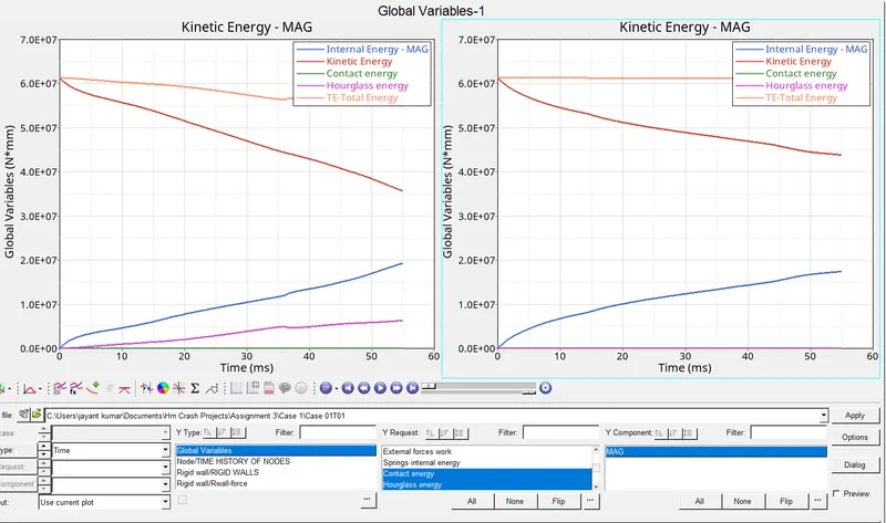
• The left hand side graph is the Case01 graph & the right hand graph is the Case02 graph.

GLOBAL VARIABLES	CASE 01 MAX VALUES	CASE 02 MAX VALUES	CASE 01 MIN VALUES	CASE 02 MIN VALUES
INTERNAL ENERGY	19285676 N-mm	17465234 N-mm	0	0
KINETIC ENERGY	61314900 N-mm	61314900 N-mm	35680184 N-mm	43792244 N-mm
CONTACT ENERGY	25441.5039 N-mm	7598.85 N-mm	0	0
HOURGLASS ENERGY	6315967.50 N-mm	0	0	0
TOTAL ENERGY	61314900 N-mm	54965860 N-mm	61314900 N-mm	61257480 N-mm

• As per the output the Case 01 has a Max Internal Energy as 19285676 N-mm and Case 02 has a Max Internal Energy as 17465234 N-mm.
• Kinetic energy are same in the maximum case for both but the minimum value is high in the case 02.
• Hourglass is zero for case 02, so it is highly recommended in this case as the case 01 is a non zero value.
•  Comparing both the result we can conclude that case 02 is very realistic and constant through all the energy conditions overally.
• The graph of the total energy is constant for case 02.

Hourglass Energy:

• It can be said as the counter for unrealistic behaviour, an hourglass energy is called when the node is getting displaced without any application of force at that point that means the element of that model is deformed but their is no strain computated.

Causes:

• insufficient properties of the element.
• Less integration points are the possiblitites that can cause hourglass effect.
• Coarse mesh flow.

To Fix:

• Improving the stiffness property to the element.
• By using fully integrated method.
• Addition of damping force where the element is seen exposed to hourglass.
• Fine mesh flow.