Assignment 3-2D Element Formulation Challenge

Aim: To compare the results of the given component with base simulation and improved shell element properties using RADIOSS.

OBJECTIVE:

1. To change the run time to 55 ms and animation step between 25 and 60.
2. To run the base simulation without any modification to element properties
3. To check the energy error and mass error checks for base simulation.
4. To plot the rigid wall forces, internal energy, hourglass energy, contact energy, total energy of the base simulations.
5. To change all the shell elements properties to recommended properties, save this as separate, rad files and run the simulation again.
6. Follow steps 4 and 5.
7. To compare all the results.

PROCEDURE:

Open the hyperworks software, and then we have to set user profile interface i.e. Optistruct or RADIOSS. Optistruct is implicit solver which handles small deformations. And RADIOSS is explicit solver which handles large deformation. So we will use RADIOSS as user interface.

First we have to import the required file i.e. Element_Formulation-Shell-3_assignment_0000.

File--->Import---->Solver Deck---->File: select file--->Import.

Once file is imported, model will look like as shown in picture below.

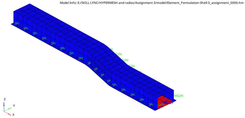
1. To change the run time to 55 ms

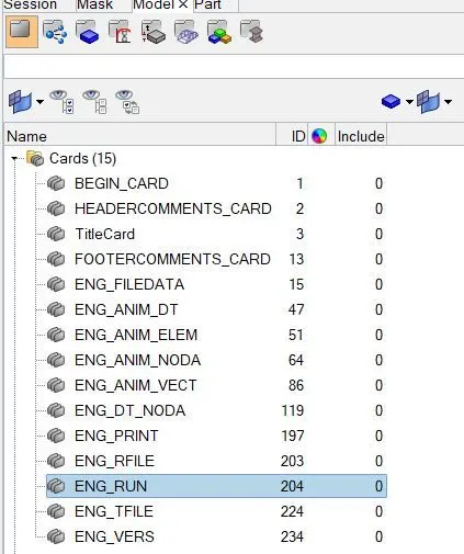
Now we have to open the model browser, and we can see the different terms such as cards, components, curves, material etc.

As per our requirement, solver have to run the model up to 55ms. To edit the run time parameter we have to follow:

Model--->Cards---->ENG_RUN---->refer below image.

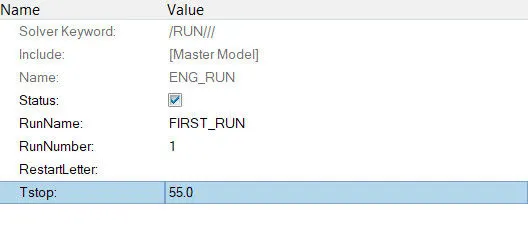
Now we have to edit the ENG_RUN parameter to 55 ms as shown in picture below.

2. To Change the number of animation steps during simulation to a minimum of 25 and maximum of 60.

So engine file has to generate animation steps between 25 and 60. So we will take a number i.e. 35. This means that solver have to generate 35 animation file with in termination time of 55 ms.

As we know, how to calculate frequency time.

Frequency time =

Frequency time =

Frequency time = 1.571

Which means a solver has to generate animation file of each 1.571 ms time interval.

Now, in order to edit the animation parameter. We have to follow:

Model--->Cards---->ENG_ANIM_DT---->refer below image.

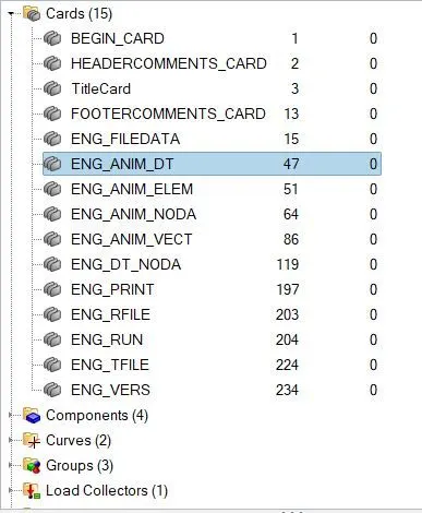
Now we have to edit the ENG_ANIM_DT parameter to 1.571 ms as shown in picture below.

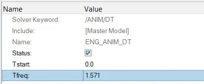
3. To run the base simulation without any modification to element properties.

Now we don’t have to edit the element properties. We have to keep it by default properties as shown in picture below.

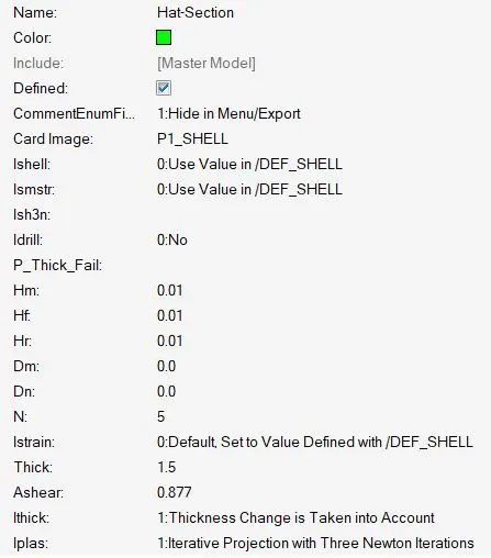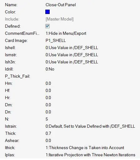Now we can check the animation by run the simulation with default properties by following:

Analysis---->Radioss

Now we have to give location to export the input file:

Options helps to choose number of cores to solve this problem, here we have chosen 4 number of cores by (-nt 4).

Then click on Radioss, and new window will get pop-up. A simulation will start to show result.

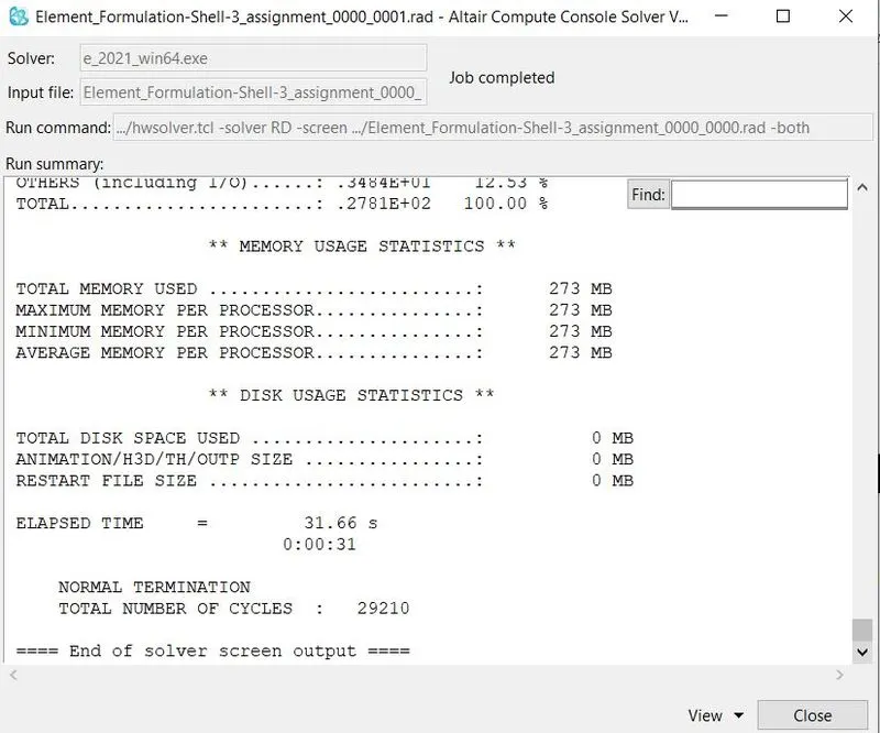
After calculating a model, solver has generated different files such as engine listing file, animation, time history and then restart file.

4. At the end of the simulation, do the energy error and mass error checks and determine whether results would be acceptable.

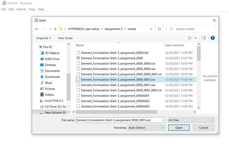
In order to check the energy error and mass error. We have to open the output file in notepad as shown in picture below.

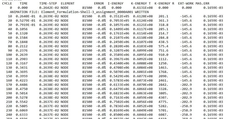
Once output file is opened, we can see the results.

At the end of simulation, we have found maximum energy error is having value of -10.3% and maximum mass error is having value of 0.165e^-3.

If the energy error lies in between range of value -15 to 5%, then results will be acceptable. If energy error is below the range, then results could be acceptable. Here we have -10.3% energy error, which is acceptable. Closer to 0%. And a mass error is coming closer to zero, which is also acceptable.

Now we have to switch from Hypermesh mode to Hyperview mode. Then we have to select the appropriated (.h3D) file. And then we have to click on Apply to view the results. Once model is opened, it will look like as shown in picture below.

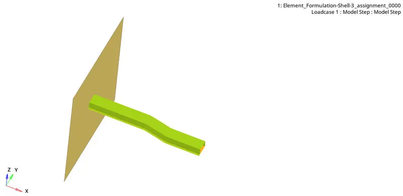
By using different animation controls, we can check and animate the results as shown in picture below.

Contour plot for Von Mises stress

Maximum stress reached upto 350 MPa over the period of 55 ms.

In the bending location, resisting strength has a little lesser then rest of area.

Now we have to switch from HyperView mode to HyperGraph 2D mode.

5. Plot rigid wall forces, internal energy, hourglass energy, contact energy, total energy of the simulations.

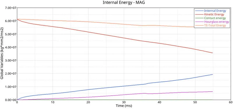
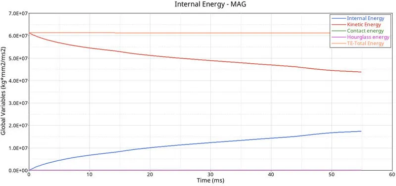
As we can see, from below graph that kinetic energy is decreasing from starting time to termination time. Because a displacement rate is reduced over a period of time. So, kinetic energy is reducing respectively.

As we know internal energy, there is no heat transfer in the system. So we only have to consider work done for calculating the internal energy. Work done is the product of force and displacement. Since a displacement is increasing over a period of time, work done will also increasing. As a result of which internal energy will also increase.

Total energy is the combination of internal, kinetic energy.

In order to build the plot graph, we have to follow steps as mentioned in picture below. First of all we have to open the required file as mentioned below.

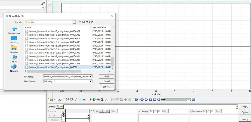
Once file is opened we have to plot the graph. In order to plot graph, we have assign different parameters as mentioned in picture below.

Once all parameters are filled, we have a required graph as shown in picture below.

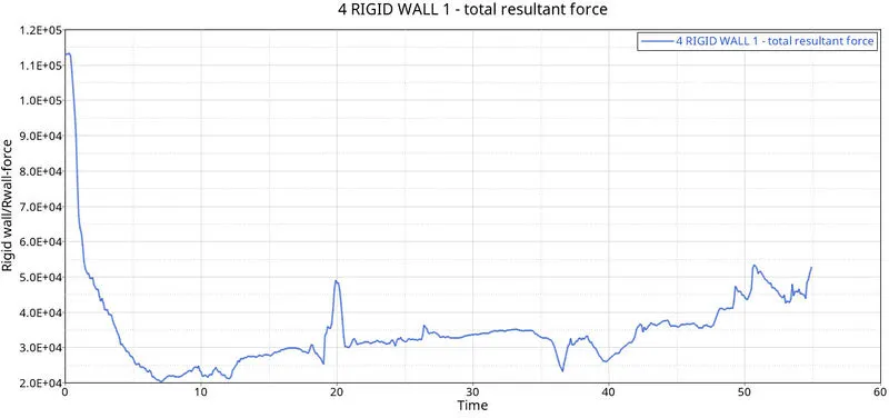
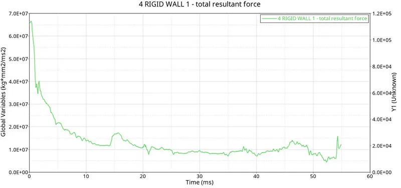
Now we have to plot the total resultant force graph. In order to plot graph, we have to follow following parameters as mentioned in picture below.

A rigid wall means that body acts rigidly alone and ignoring deformation. Once all parameters are filled, we have a required graph as shown in picture below.

6. Change all the shell elements properties to recommended properties, save this as separate, rad files and run the simulation.

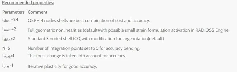
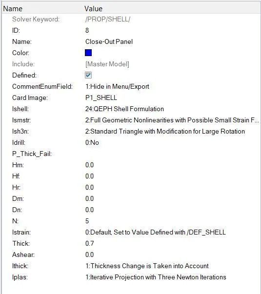
Now, we have to change the default shell elements properties to recommended properties. So, recommended shell elements properties are shown in picture below.

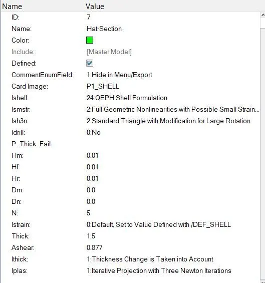
To change default shell elements properties to recommended properties, we have to follow steps mentioned below.

So, in order to run the simulation, we have to follow same steps as mentioned above. Once simulation is done, then we have to calculate mass error and energy error as mentioned in picture below.

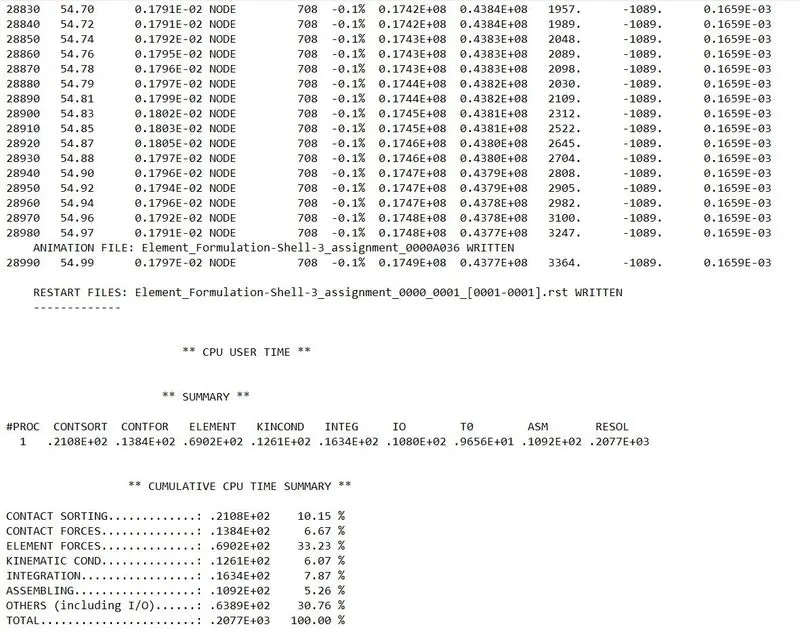
From above picture we can see the energy error is having value -0.1% and mass error is have same value as we got for above step with default shell element parameters i.e. 0.1659e^-3.

Contour plot for Von Mises stress

As sane, Maximum stress reached up to 350 MPa over the period of 55 ms.

In the bending location, model is deforming heavily as compared to above case.

Once required graphs has plotted as shown in picture below. We can observe that after change default properties to shell elements properties there is no change in internal energy and kinetic energy. But we can see there is no hourglass energy has generated. This is because we have used QEPH element formulation. As we know QEPH 4 node shells are best combination of cost and accuracy.

And total energy is maintained at higher as compared to previous case. This is because there is no hour glass energy has generated.

Similarly, graph has been plot for rigid wall total resultant force as mentioned in picture below.

CONCLUSIONS

1. Simulation has been done for same model with default shell element properties and with modified required shell elements properties. As we can see difference there is no hourglass deformation is formed when we have used model with required shell element properties and also maintained the results accurate.
2. So, we can conclude results are effective when shell elements are modified because of no hourglass deformation because QEPH 4 nodes shells has been used.

---------------------------------------------------------------------------------------------------------------------------------------------------------------------------------------------------------------

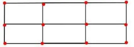
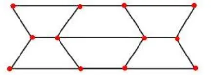
Hourglass deformation:

When the elements in model deform but the strain energy is not computed for that deformation then it results in hourglass deformation. Usually this can be clearly see in post processing stage where the elements will have zig zag formation.

Normal elements:

Elements with Hourglass effect:

To fix hour glass deformation:

1. Stiffness can be added to the reduced integration element at the material level where this hourglass has occurred.
2. A damping force can be added at the deformation, depending upon the deformation the force will be computed.
3. By using fully integrated elements, hourglass deformation can be avoided.
4. Mesh refinement also helps in avoiding this hourglass deformation.