Assignment 3-2D Element Formulation Challenge
Aim - To perform the analysis for the given mesh model with connections. Solve the model in two cases, the effect of hourglass energy and energy error can be determined with the given propertis.
Objectives
Case I
Comparison of results with base simulation and improved shell element properties
1.Using the crash beam file from the previous assignment, change the run time to 55 ms.
2. Change the number of animation steps during simulation to a minimum of 25 and maximum of 60.
3. Run the base simulation without any modification to element properties.
Case I
Recommended properties:
| Parameters | Comment | |
|
Ishell =24 |
QEPH 4 nodes shells are best combination of cost and accuracy. | |
|
Ismstr=2 |
Full geometric nonlinearities (default)with possible small strain formulation activation in RADIOSS Engine. | |
|
Ish3n=2 |
Standard 3 noded shell (C0)with modification for large rotation(default) |
|
| N=5 | Number of integration points set to 5 for accuracy bending. | |
|
Ithick=1 |
Thickness change is taken into account for accuracy. |
|
|
Iplas=1 |
Iterative plasticity for good accuracy. |
Introduction
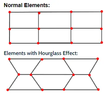
Hourglass Deformation - For the under-integrated shell element, displacements and forces may exit for each node of the element, like the sum of all these forces and displacements give null strain and stress on the integration point of the element.
This problem exist only for under-integrated element.
Typical hourglass deformation:
Hourglass energy, which is work done by the forces calculated to resist hourglass modes, takes away from physical energy of the system.
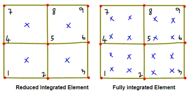
As above shown figure the effect of hourglass energy can be determined by 2 types
- Reduced integrated method- 2nd node will get displcement by effecting the surrounded nodes of 5,4,1 then it will create the hourglass effect for the mesh model.
- Fully integrated method- The elements of 4 nodes will be gets displaced at a time in the elements, avoid the hourglass effect.
Procedure
In this files there is having the starter file and engine file.
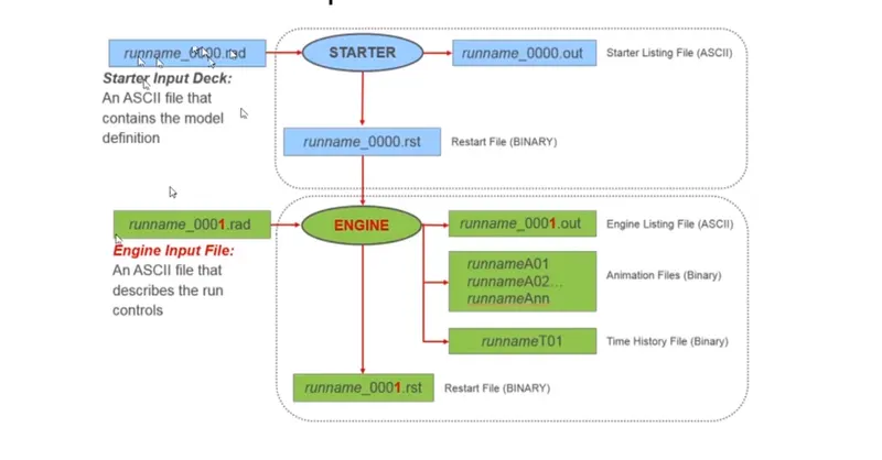
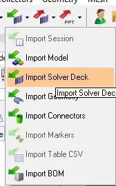
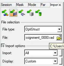
Import the starter file from the solver deck as shown in below and import in to GUI.
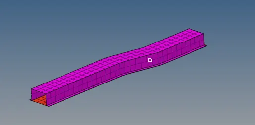
The mesh geometry imported from the solver deck as shown in below.
Case I
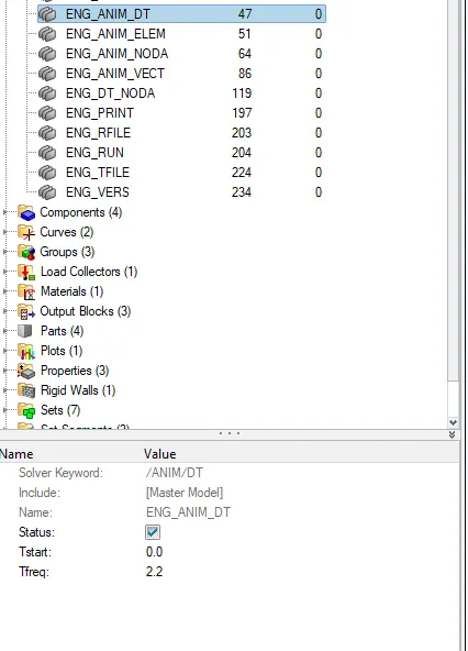
The select the mesh model collector and ANIM_DT file find the values for the Tfrq
In animation steps choose the no between 25 to 60.
Tfrq=Run Time/No of animation steps
=55/25
=2.2
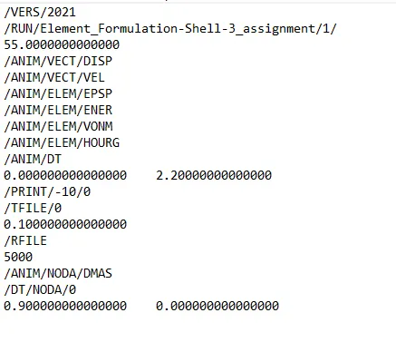
The values for the Tfrq can be assign in the file card.
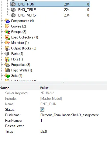
Assign the engine run value as 55 for stoptime period.
For assigning the both the parameters and run for the Radioss analysis with proper save in the file as shown in below. To increase the speed of analysis is assigning the -nt 4 used in option.

After done simulation open the 0001.rad file all energy error and mass error can be seen below. The energy error will be acceptable -15 to +5 in the accept.
The below shown rad file shows -10.3% of energy error and its acceptable.

The other rad file will show the assigning the parameters values.
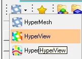
After analysis go for the hyperview to run the animation file.
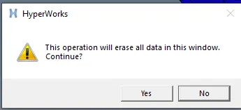
Select it as yesand the mesh model turns into the animation mode.
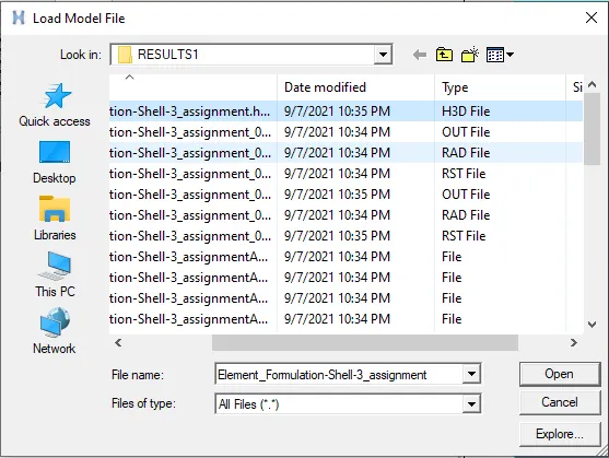
By selecting the H3D file and open in to the hyperview.
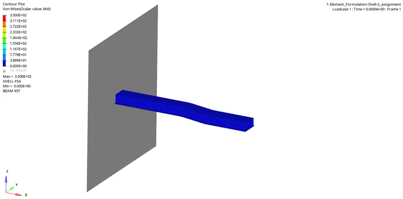
Apply after importing the file and the mesh model is ready for the animation as below shown.

The mesh model have the all spot weld connections and also have object to hit as shown in below
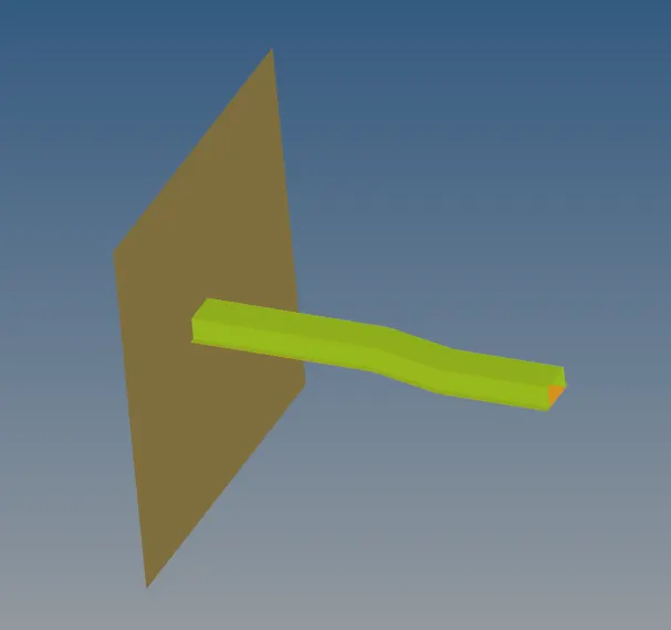
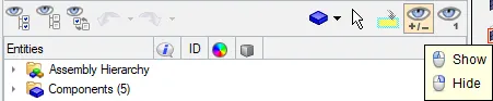
By selecting the hide botton the component will get hide.
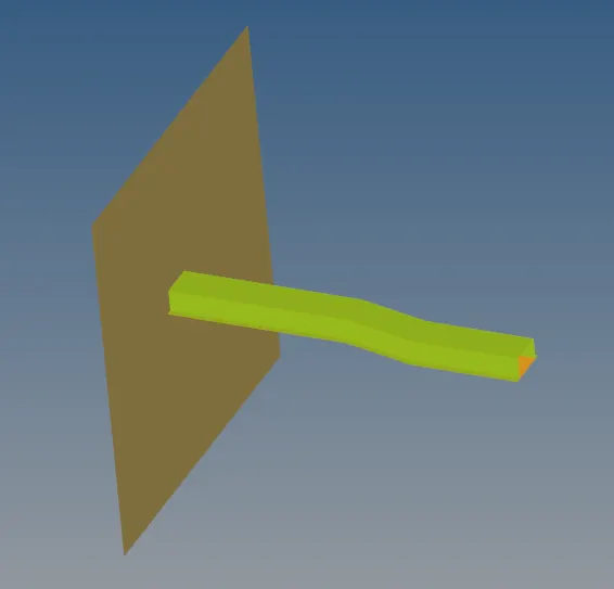
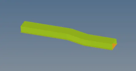
The below shown images before and after hiding the object as shown in below.
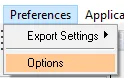
Select the preferences with options of visualization.
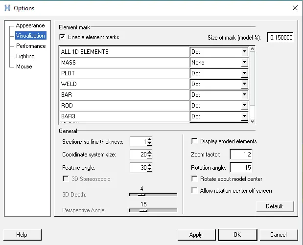
Slect the in the visualization and set the size for mark as 0.15, also select the all elements as Dot and apply.
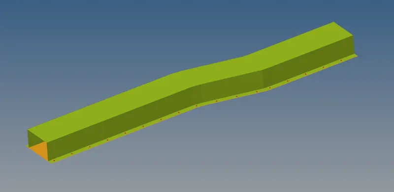
Then play with the animation file in hyperview.
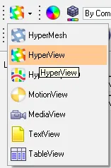
Select the h3d file and import it, and apply.
Then play with the animation file in hyperview.
The pages can be splitted for 4 so that perform the other operations in to account. Use the expand and reduce the window.
On the basis of the animation, plot the graph for the various energy for the given component.
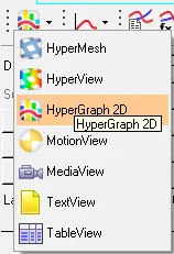
The shared screen is turns in to graph mode as shown in below.
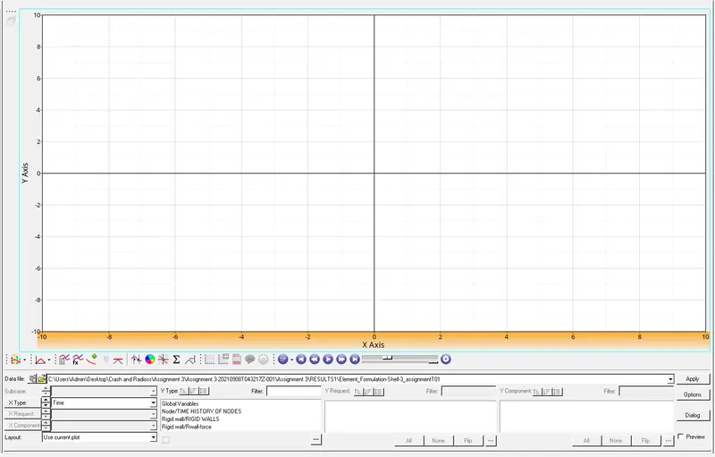
Select the file as the T01 is import in to the GUI and apply it.

By selecting the global varables, select the kinetic energy, inernal energy, total energy, hourglass energy and contact energy can be plotted and select apply.

Graph 1
The below shown the all forces of various energy graph is to be plotted.
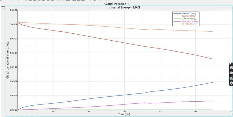
1)As shown in garaph the kinetic energy is high initially and kanetic energy is decreases w.r.t time. The kinetic energy is directly proportional to the mass and velocity.
As the mass and velocity decreases the kinetic energy also decrease at time period of 55 ms. The effect of the K.E in graph shown in above.
K.E= 1/2*mv^2
=1/2*503881.261*(-15.6)^2
=61312240
=6e7 Nm
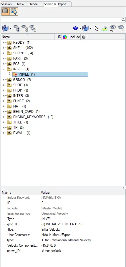
The kinetic energy have mass and velocity has been self assigned in the file.
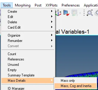
The mass details can be shown in tools and in that mass details. Considering the total mass.
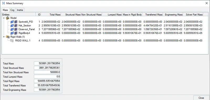
The velocity has been self inserted in solver already in INIVEL and velocity of componenet.
2) For the internal energy there is initially no deformantion in the component so, in the graph has been started from origine.
Gradually there is change in the deformantion in the model so graph has been increases from origine to some height w.r.t time.
Similarly for the rigidwall force also plot the graph for that.
ΔU = Q + W
| ΔU | total change in internal energy of a system, |
| q | heat exchanged between a system and its surroundings |
| w | work done by or on the system |
3) Hour glass energy showing some error while analysis the model in radioss so, due to reduced integrated method it was showing some error so the hourglass effects shown on the graph.
Hourglass energy = 5% of internal energy.
4) Total energy has been taking count of all resultant energies and and it has been start from the whre the error energy will occure. The other way of finding the energy error is in kinetic
energy reduce the 10% of K.E becomes energy error.
Energy error= K.E - 10% K.E
5) Contact energy - The energy has beeen generating from the contact between 2 surfaces and by compering this it has been negligible.
Graph 2
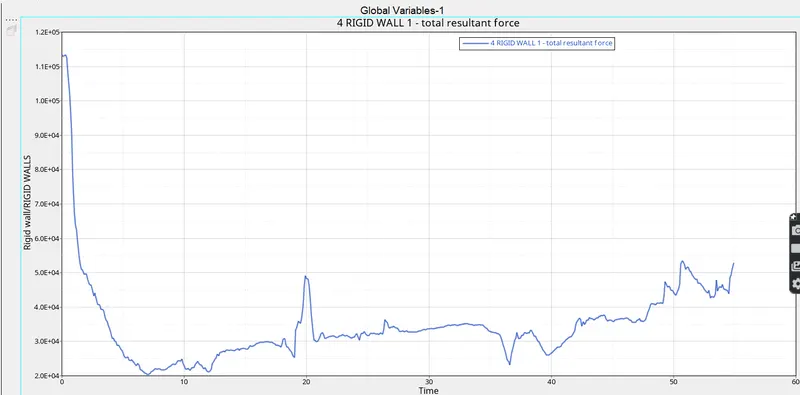
For regidwall forces of resultant forces can plot the graph as below shown in the image when the speed of sound is equal to the speed of the waves.
To create graph for the regid walls the total resultant forces can be select.

Initially the speed of sound will be more due to the displacement of model start gradually it was decreasing w.r.t time period as shown in the graph
Case II
The select the mesh model collector and ANIM_DT file find the values for the Tfrq
In animation steps choose the no between 25 to 60.
Tfrq=Run Time/No of animation steps
=55/25
=2.2
The values for the Tfrq can be assign in the file card.
Assign the engine run value as 55 for stoptime period.
For case II there is not assigning the parameters so, using the fully integreted nodes properties can be given
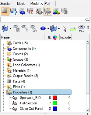
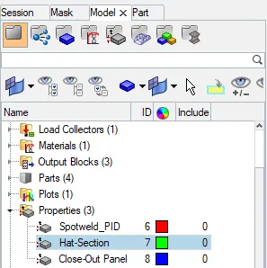
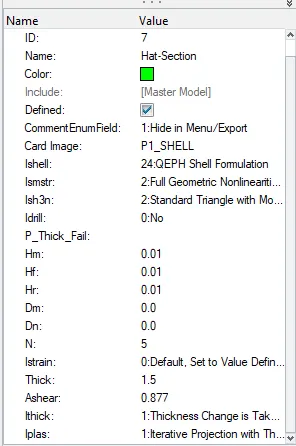
The given properties hat-section can be select the assign the given properties in to the same as given for case II.
Assine in to the prperty card as Ishell =24 Ismstr=2 Ish3n=2 N=5 Ithick=1 Iplas=1.
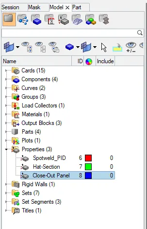
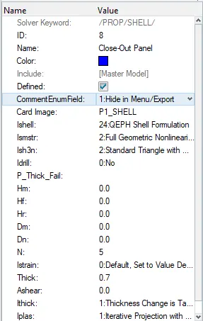
Also assine in to the prperty card of close out panel as Ishell =24 Ismstr=2 Ish3n=2 N=5 Ithick=1 Iplas=1.
For assigning the both the parameters and run for the Radioss analysis with proper save in the file as shown in below. To increase the speed of analysis is assigning the -nt 4 used in option.
After done simulation open the 0001.rad file all energy error and mass error can be seen below. The energy error will be acceptable -15 to +5 in the mantain.
For this case the energy error should be -0.1% so, its acceptable.
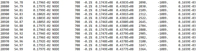
The other rad file will show the assigning the parameters values.
After analysis go for the hyperview to run the animation file.
Select it as yes and the geometry turns into the animation mode.
By selecting the H3D file and open in to the hyperview.
Apply after importing the file and the mesh geomety is ready for the animation as below shown.
The mesh geometry have the all spot weld connections and also have object to hit as shown in below.
By selecting the hide botton the component will get hide.
The below shown images before and after hiding the object as shown in below.
Select the preferences with options of visualization.
Slect the in the visualization and set the size for mark as 0.15, also select the all elements as Dot and apply.
Then play with the animation file in hyperview.
Select the h3d file and import it, and apply.
Animation file has been shown in below.
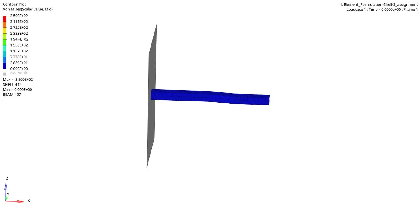
The pages can be splitted for 4 so that perform the other operations in to account. Use the expand and reduce the window.
On the basis of the animation, plot the graph for the various energy for the given component.
The shared screen is turns in to graph mode as shown in below.
Select the file as the T01 is import in to the GUI and apply it.
By selecting the global varables, select the kinetic energy, inernal energy, total energy, hourglass energy and contact energy can be plotted and select apply.
Graph1
The below shown the all forces of various energy graph is to be plotted.
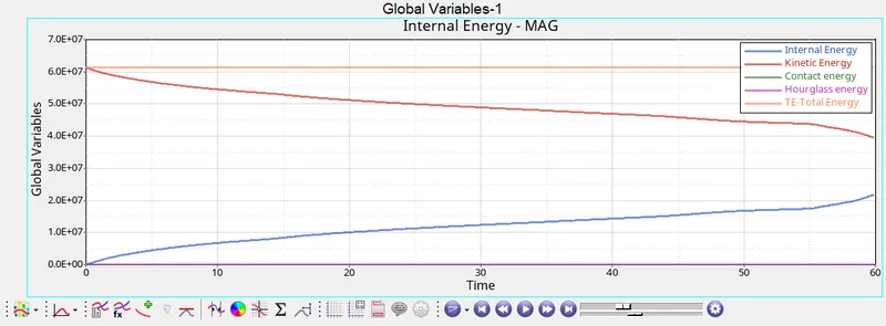
1) In the garaph shown the kinetic energy is high initially and kanetic energy is decreases w.r.t time. The kinetic energy is directly proportional to the mass and velocity.
As the mass and velocity decreases the kinetic energy also decrease at time period of 55 ms. The effect of the K.E in graph shown in below. For kinetic energy the parameter has been
already assined
K.E= 1/2mv^2
2) For the internal energy there is initially no deformantion in the component so, in the graph has been started from origine.
Gradually there is change in the deformantion in the model so graph has been increases from origine to some height w.r.t time.
Similarly for the rigidwall force also plot the graph for that.
ΔU = Q + W
| ΔU | total change in internal energy of a system, |
| q | heat exchanged between a system and its surroundings |
| w | work done by or on the system |
3) Hour glass energy showing some error while analysis the model in radioss so, due to fully integrated method it was shows there is not have any effects for hourglass effects shown on the graph.
Due to that the graph is on straight line.
4) Total energy has been taking count of all resultant energies and and it has been start from the whre the error energy will occure. The other way of finding the energy error is in kinetic.
energy reduce the 10% of K.E becomes energy error. In this case the energy error will be reduced because of assigning the standerd parameters.

5) Contact energy - The energy has beeen generating from the contact between 2 surfaces and by comparing to this it has been negligible.
Graph 2
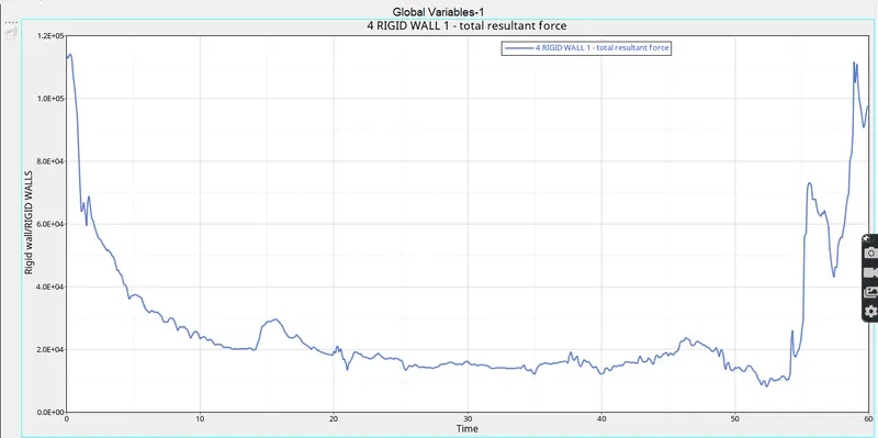
For regidwall forces of resultant forces can plot the graph as below shown in the image when the speed of sound is equal to the speed of the waves.
Initially the speed of sound will be more due to the displacement of model and decreasing speed. At the end of the model is hit again to the object and create the speed of sound so, graph is gradually
increases w.r.t time period as shown in the graph.
Comparision of case I and case II
| case I | case II | |
| KINETIC ENERGY | 0.3563E+08 | 0.4377E+08 |
| INTERNAL ENERGY | 0.1932E+08 | 0.1749E+08 |
| ENERGY ERROR | -10.3% | -0.1% |
| HOURGLASS ENERGY | The hourglass energy is gradually increases due to the reduced intigrated elements | In this the hourglass enrgy can be remains constant because of assigning the standard parameters values of Pshell(QEPH) elements. |
| Contact energy | The contact energy will produces with mating the 2 objects is negligible | The contact energy will produces with mating the 2 object is less. |
| Regidwall forces | Initially with high force will apply after it becomes gradually decreasing. | Initially with high force will apply after it becomes gradually decreasing. At finally the model is hit with object create with incrasing force as shown in graph |
Conclusion
To performing of this analysis with 2 cases concluded that
In case I there is not have assigning any staderd parameters on before analysis the to avoid the hourglass energy and total energy error results in to creating the houglass error and energy error.Bacuse of the reduced integrated elements in the model.
Similarly for case II there is assignig the standerd parameters for before analysis so, the effect of hourglass energy error and total energy error will be avoid in the given model. Because of introducing the fully intigrated standerd properties has been assigned.