Crash Analysis for a given Specimen before and after Element Property Change in RADIOSS
Assignment 3 Report.
- Objective: 1. To change the Run time of the model.
2. To change the Frequency of the simulation such that the number of animation files is between 25 and 60.
3.To check the Energy error and Mass Error in the simulated model.
4. To plot the graphs of Wall forces and internal energy, hourglass energy, contact energy and the total energy of the simulation.
5. To run and compare the simulation results for the changed Shell element properties in the model. - Procedure:
1. The very first step when we have to change the run time in the model we need to firstly import the model. To import it, we need to click on the Import button and use the file option in it.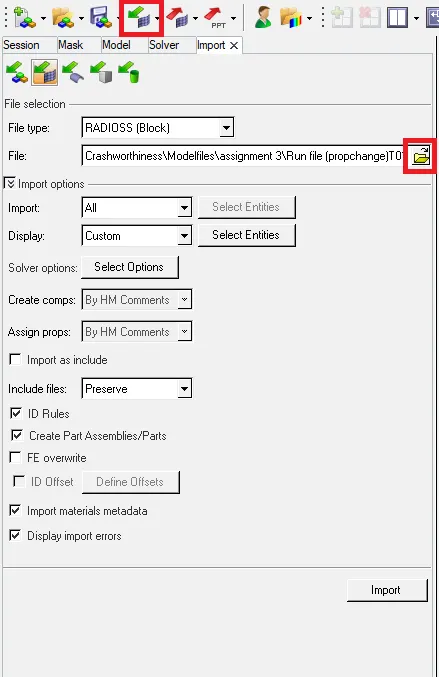
Import command.
2. After the file is imported, then we need to select the Cards file in the Model tab and use the "ENG_RUN" file in it. Here we need to change the Tstop time to 55 as stated in the Question.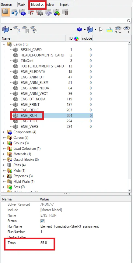
To change the Run time of a Simulation.
Like this we can terminate the simulation at any instance we want. (55ms in this case)
3. After the Simulation time was changed, we need to the number of Animation Files somewhere in between 25 and 60 as stated. So to alter the number of Animation files, we need to change the Tfreq in the "ANIM_DT" file. Since we already know that :
Run time / Number of Animation files = Tfreq
In our case, the Run time will remain the same. i.e. 55ms and the number of animation files can be anything between 25 and 60. So I chose the frequency as 2.0 and did the simulation.
So, according to this simulation 29 Animation Files.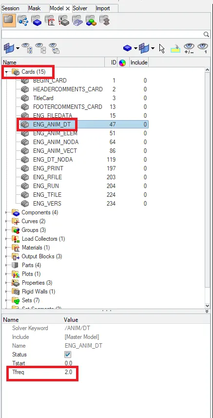
Changing the Tfreq according to Animation files required.
4. To run the simulation, we need to use the Analysis tab and use the Radioss option in it.
Analysis -> Radioss
Radioss Command
After selecting the file, we then need to run it and then check the results that we get.
5. To see the Energy error and the mass error for the simulation that we just performed, we need to open the Engine output file that we get after the simulation is performed. This file will be saved in the same location where we have saved all the other Animation files. This output file will be in the format of "filename_0001.out". once we open this file, we then need to check the Energy error for all the cycles in the model.
An example of the Energy error and the mass error is shown below: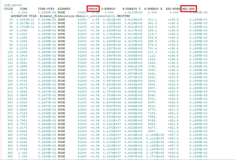
Energy Error before changing the properties.
Generally the energy error should be between -5% to +15%. Anything below or above this value means that there are some issues in the model that are needed to be fixed. Like this, we can check the energy and mass error in the model.
5. To change the properties in the model, we need to use the "Properties" card and change the PSHELL Elemental Properties.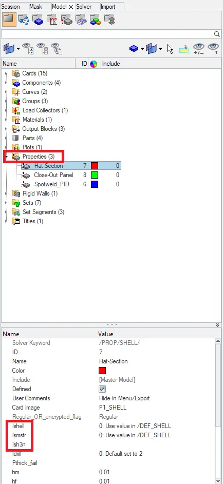
Changing the properties of the element.
Values of these properties are to be changed accodringly. For example the Value of Ishell is to be changed from 0 to 24. This change means that the Elemental Formulation changes to "Fully integrated".
Using this tab, we can change all the properties, some of which include Ishell, Ismstr, Ish3n etc. Changing these properties implies that we change how the formulation of the elements and change how the calculation across all the elements will take place. This can mean that we may have increased the computational time but also increased the Accuracy of the simulation. After the property was changed, we saw that the Energy error also drastically reduced and was much more controlled.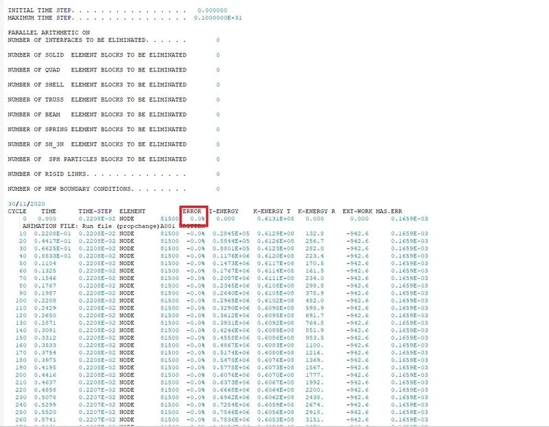 Energy Error for when we change the property.
6. After the Properties were changed, we need to save this as a seperate file rerun the simulation using the same process. We get very different results when we comapre the plots of the two simulations.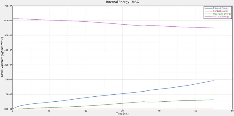
Without change of properties.
In this graph, we can see that the curve representing total energy(pink line) is going down, meaning that the total energy of the system is decreasing. This means that the Energy is being dissipated in the entire system. This can be confirmed with the rise in the values of the Hourglass Energy(green line). The curve representing the Hourglass energy is gradually rising up and becoming stable as time passes.
Hence the reduction in the total energy of the model can be accounted in the rise of the Hourglass energy.
As for the Internal Energy, the curve is rising continously as the Deformation in the specimen is continually increasing with the passage of time.
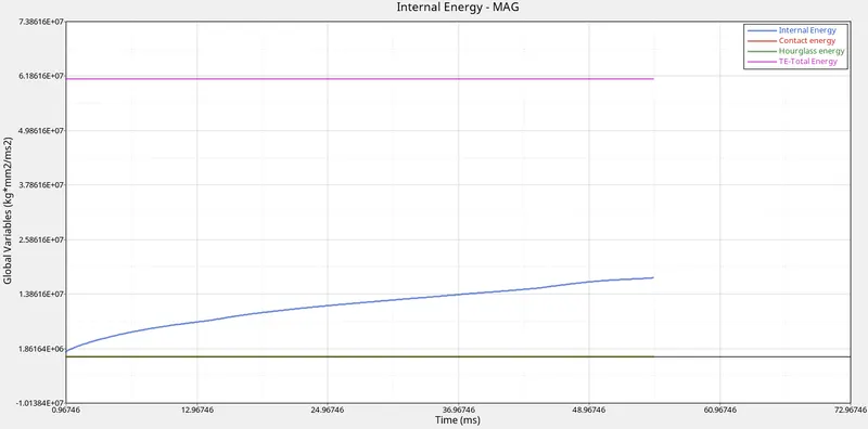
With property change.
This graph represents the plots for when we have changed the properties for the Shell elements. We can clearly see that the Total Energy curve(Pink line) remains constant throughout the simulation. And even the Hourglass Energy curve(green line) remains constant. This means that when we change the properties of the elements the simulation method and results change as well.
The internal energy is this case is also continuously increasing as the Deformation in the specimen is also increasing as time progresses in the simulation.
Now as for the normal forces on the model. The graphs are as follows: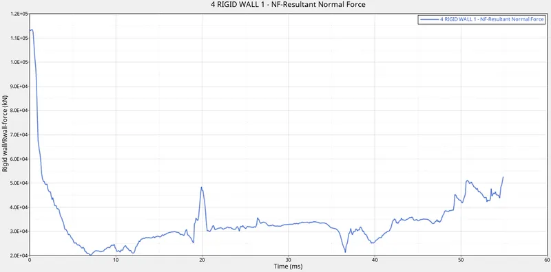 without property change
This is the graph that we get when we plot the Normal forces on the wall. We can see that the speciment is breaking and making contact with the wall. And we observe that the speciment is crushing into the wall, we see that the contact between the wall and the specimen increases.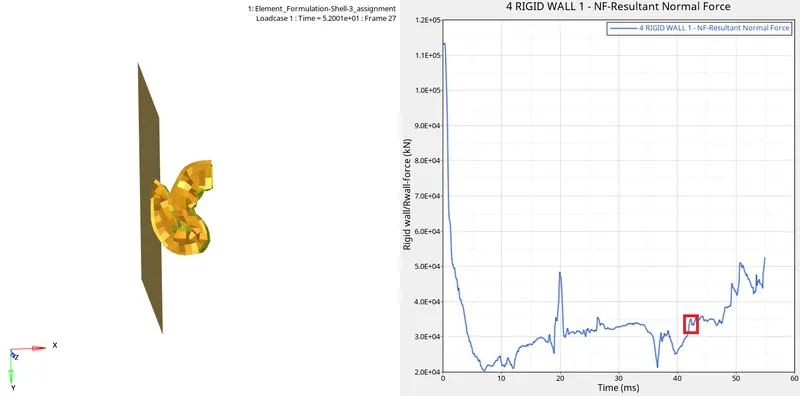 Graph showing the rise in Normal forces.
The crushing and failing of the structure begins after the marked point in the graph. After this point the specimen crashes into the wall and the contact between them increases and there is a rise in the normal forces which can be seen in the graph.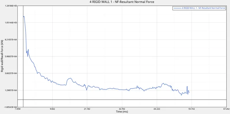 With property change.
When we see the graph for the Normal forces when the property was not changed, we can see all the various spikes in the graph. These spikes represent for when the specimen was came in contact with the wall. Whenever we observe a spike in the graph, it indicates that the Specimen has made contact with the wall. As we can see from the simulation video, the specimen is making contact contact with the wall in some point of time and at some other instance, the contact with the wall is decreasing therby a reduction in the normal forces. This is happening because the specimen is buckling and pivoting at one point on the wall. As The simulation progresses, and the specimen is getting crushed into the wall, the side portion of the specimen is coming in contact with the wall hence the normal forces fluctuate as shown in the graph. But in this case the forces relatively constant after the drop in its value.
For reference purposes, I have attached the GIF File as well: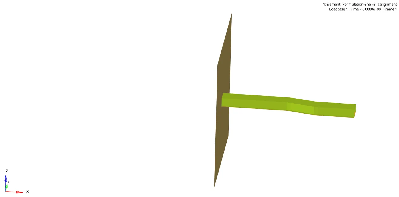
Without property change.
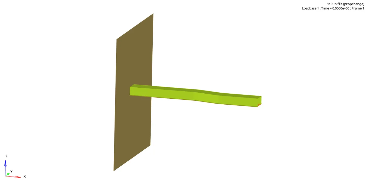
With property changed.
We can clearly see that the entire simulation changes as we change the properties of the elements.
- Conclusion: In conclusion I would like to state that this assignment helped me understand how to plot the required graphs and how to study them as well.