Assignment 2-RADIOSS Engine File Editing & 3D Meshing Challenge

1. Speed of sound in steel rail = 5188.7852 mm/ms
2. Time taken by shock wave = 0.1927 ms
3. Time for sound to travel length of rail = 0.1927 ms

1. Introduction

Radioss is an explicit solver widely used in crashworthiness analysis for passenger cars. The input file for the radioss solver is written as a text file and all the information are present in the form of different keywords and their values. The good thing about it being a text file is that it can be easily edited in any text editor like notepad. The radioss file is madeof blocks, each block defines one feature: a set of nodes, elements, a material etc. Each block starts with a "/" followed by a keyword and ends at the beginning of the next block.

The contents of each block is entered as a formatted lines of 100 characters divided into 100 fields of 10 characters.

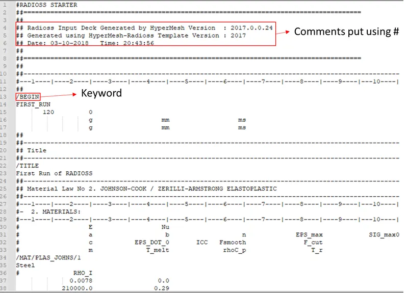
Fig 1.1: Snippet of a radioss keyword file

There are two sets of files called Starter and engine files. The figure below shows the structure of these files.

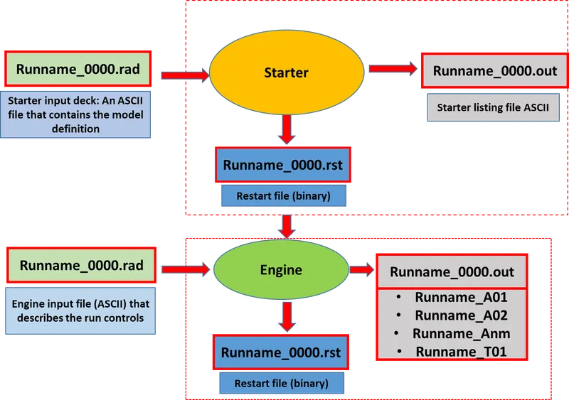
Fig 1.2: Different files of a radioss solver deck

Here the engine files refer to the starter input file which also contains the solution controls.

2. Assignement part 1

An input file containing a model of a 1000 mm rail components crashing to a rigid wall is given and following changes need to be made in it:

1. Check the material properties of the rail component and calculate the speed of sound in steel rail=_______

2. The length of the rail is about 1000 mm.calculate the time takes for a shock wave to travel from one end of the rail to the other.

3.Time for sound to travel length of rail=______

4.Edit the engine file so that the stress wave can be monitored, moving from one end of the rail to the other during impact -this will require a termination time equal to the time it takes for the sound to travel the length of the rail(set on/RUN card)

5.Set the frequency of animation output to a time that will give 20 animation steps(/ANIM/DT)

6.Change /print -10.

2.1 Solution part 1

The given file 0000.rad file was imported into the hypermesh and material data was looked as shown in the attached figure.

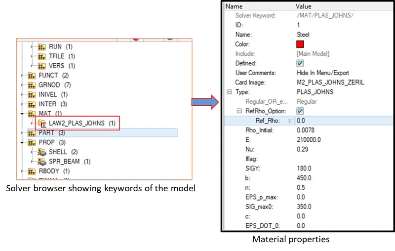
Fig 2.1.1: The snapshot from the solver browser showing material properties

As clear from the above figure a M2_Plas_Johns_Zeril card was used which is similar to piecewise linear plasticity model used in LS-Dyna. The unit system followed in the model is [g-mm-ms] which tells us the different values to be : Density = 7800 kg/m^3 , Young's Modulus = 210 GPa, Poisson's Ratio = 0.29, Yield stress = 180MPa.

The evaluation of speed of sound in solids can be made using the formula:

It gives us c=5188.745 m/s and based on 1000 mm length the time for a wave to propagate through the rail comes out to be t=l/c or t= 0.193 ms.

Next, we need to change the values in the input file :

1. changing the run time:

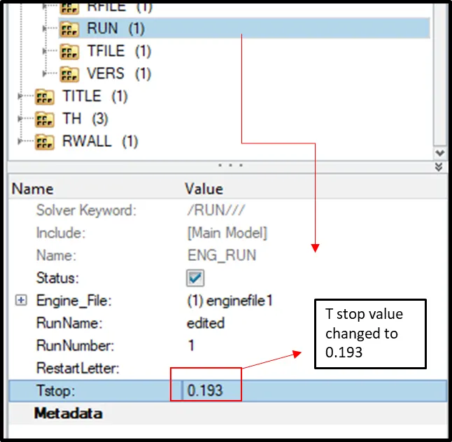
Fig 2.1.2: The run time changed to 0.193 ms

After that, the frequency of animation output needed t be changed so that a total of 20 animation steps are recorded by the solver. Dt = total runtime /no. of animation files. This leads to the Tfreq value being changed to 0.00964 ms in the /ANIM/DT card.

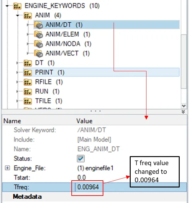
Fig 2.1.3: The Tfreq value changed in the ANIM/DT card

Finally the result printing value needed to be set after 10 cycles. This was done by changing the N_print value to -10 as shown in the below figure.

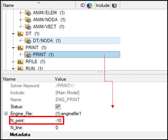
Fig 2.1.4: The Tfreq value changed in the Print card

3. 3D meshing of components

3.1 The Arm Bracket

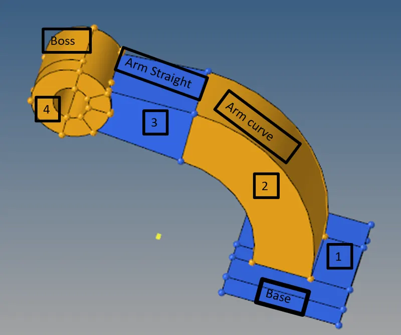
Fig 3.1.1: The arm bracket geometry

It contains four different sections as shown in the attached figure. It was asked to perform hex meshing on it with a target element size of 10 mm. The process for generating mesh was using the solid map, spin and line drag options available in the hexa meshing panel. First 2D mesh was generated on the one of the face which then needed to be dragged in the case of line drag is used. In case, solid map is used a matching 2D mesh needs to be done on the opposite face with exact number of elements. For the curved portion spin option was used to generate hexa mesh. Face option comes handy while performing line drage or solid map. It generates 2D mesh on the faces of the solid map which can be used in the next operation.

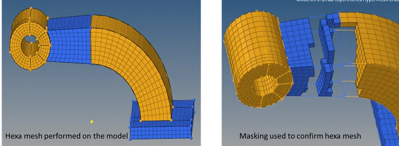
Fig 3.1.2: The meshed model

After that we need to ensure the connectivity between the elements specially at the interfaces. This can be done using edges option present in the tool menu. Basicaly, equivalence of the nodes is checked and then we go on checking the presence of edges which indicate presence of non-equivalenced nodes.

3.2 The Housing model

A model of a hub and its housing was given and it was asked to perform tetra mesh on it with a target size of 5 mm. The method adopted was to initially create a tria mesh of 5 mm on all the surfaces which was then converted to tria mesh using the tetra mesh panel.

The tet collapse was checked and kept below 0.15 as instructed for the exercise.

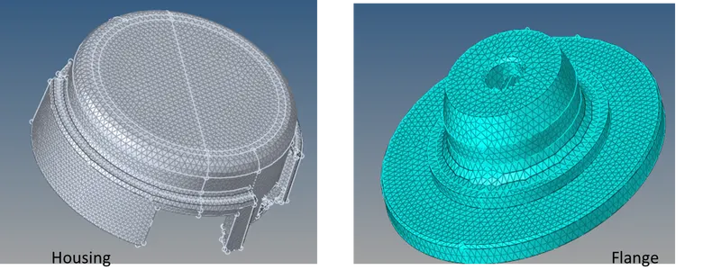
Fig 3.2.1: The tetra mesh generated on the housing model