Air Standard Cycle
AIM: To Write code in MATLAB that can solve an otto cycle and plot PV diagram.
REQUIREMENTS :
- To create a PV diagram using MATLAB code.
- To find the thermal efficiency of the engine.
DESCRIPTION
Air standard Otto cycle is used for the SI Engines (Spark Ignition Engine).
The Ideal Otto cycle consists of the four processes which are as below.
1–2 Reversible Adiabatic compression (Or) Isentropic Compression.
2–3 Constant Volume Heat Addition.
3–4 Reversible Adiabatic Expansion (Or) Isentropic Expansion.
4–1 Constant Volume Heat Rejection.
When the piston in the cylinder of the Internal Combustion Engine (SI Engine) moves from BDC (i.e Bottom Dead Centre) to TDC (i.e Top Dead Centre) the Pressure and volume Relatively change, which is represented on the Diagram known as PV-Diagram. The ideal PV-Diagram can be seen below.
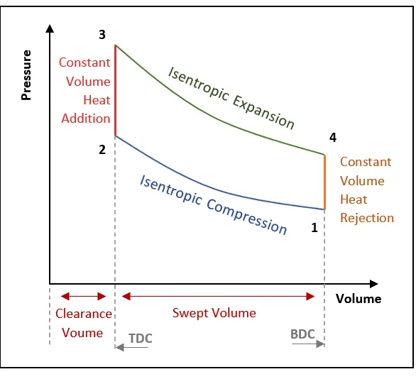
Otto Cycle works on four processes, which commences with intake stroke where the mass of air is pushed into the piston at unvarying pressure. The second step is compression stroke, where isentropic compression takes place. It is the actual time when the mixture of fuel and air is compressed. At this point, the cylinder will move from bottom dead center to the top.
Then comes the ignition phase where the piston respites at the top dead center, for a while. Heat is now pushed into the system that burns the mixture of air and fuel already present there. It leads to acceleration in the pressure, keeping volume steady. It proceeds to expansion stroke, and heat rejection phase later on, which is followed up by the exhaust stroke in the end.
Defining State variables :
State variable at point 1:
i.Initial pressure and temperature
P1 = 101325 and T1 = 500K
ii.Engine geometric parameters
Bore = 0.1
Stroke = 0.1
Connecting rod length(cond_rod) = 0.15
compression ratio(cr) = 12
iii. Swept volume is the volume of the cylinder i.e., by bore and stroke
v_swept = (pi/4)*bore^2*stroke
v_clearence = v_swept/(cr-1)
State variable at point 2:
i. calculating pressure at point 2(P2)
PV^gamma defines isentropic compression process
P1V1^gamma = P2V2^gamma
P2 = P1*(V1/V2)^gamma
V1/V2 = cr
P2 = P1*(cr)^gamma
ii.Calculating temperature T2
For computing temperature(T2) in state 2 we are using ideal gas law
(P1V1)T1 = (P2V2)T2
Hence T2 = P2*V2*T1/P1*V1
State variable at point 3:
i.It represents the end point of the constant volume combustion and hence V3 = V2
ii. Calculating pressure at point 3
Using the ideal gas law : P3 = P2*(T3/T2)
State variable at point 4:
i. calculating volume at point 4 (V4)
V4 = V1
ii. Calculating pressure at point 4
P4 = P3*(V3/V4)^gamma
After defining all the state variables an initial program can be written as
 clear all
 close all
 clc

 %Inputs
 gamma = 1.4
 t3 = 2300

 % state variables
 p1 = 101325
 t1 = 500

 %state engine variables
 bore = 0.1;
 stroke = 0.1;
 cond_rod = 0.15;
 cr = 12;

 % calculating the swept volume and the clearence volume
 v_swept = (pi/4)*bore^2*stroke;
 v_clearence = v_swept/(cr-1);

 v1 = v_swept+v_clearence
 v2 = v_clearence

 % state variables at state point 2
 % p1*v1^gamma = p2*v2^gamma
 % p2 = p1*(v1/v2)^gamma
 % p2 = p1*cr^gamma
 p2 = p1*cr^gamma

 % p1v1/t1  = p2v2/t2
 % t2 = p2*v2*t1/(p1*v1)
 t2 = p2*v2*t1/(p1*v1)

 % state variables at state point 3
 v3 = v2

 % p3v3/t3 = p2v2/t2 | p3 = p2*t3/t2
 p3 = p2*t3/t2

 % state variables at state point 4
 v4 = v1

 % p3v3^gamma = p4v4^gamma  | p4 = p3(v3/v4)^gamma
 p4 = p3*(v3/v4)^gamma

 figure(1)
 hold on
 plot(v1,p1,'*','color','k')
 plot(v2,p2,'*','color','k')
 plot(v3,p3,'*','color','k')
 plot(v4,p4,'*','color','k')
 xlabel('volume')
 ylabel('pressure')

 figure(2)
 plot([v1 v2 v3 v4],[p1 p2 p3 p4],'color','b')
We got a PV diagram having four points in which it represents the state points.
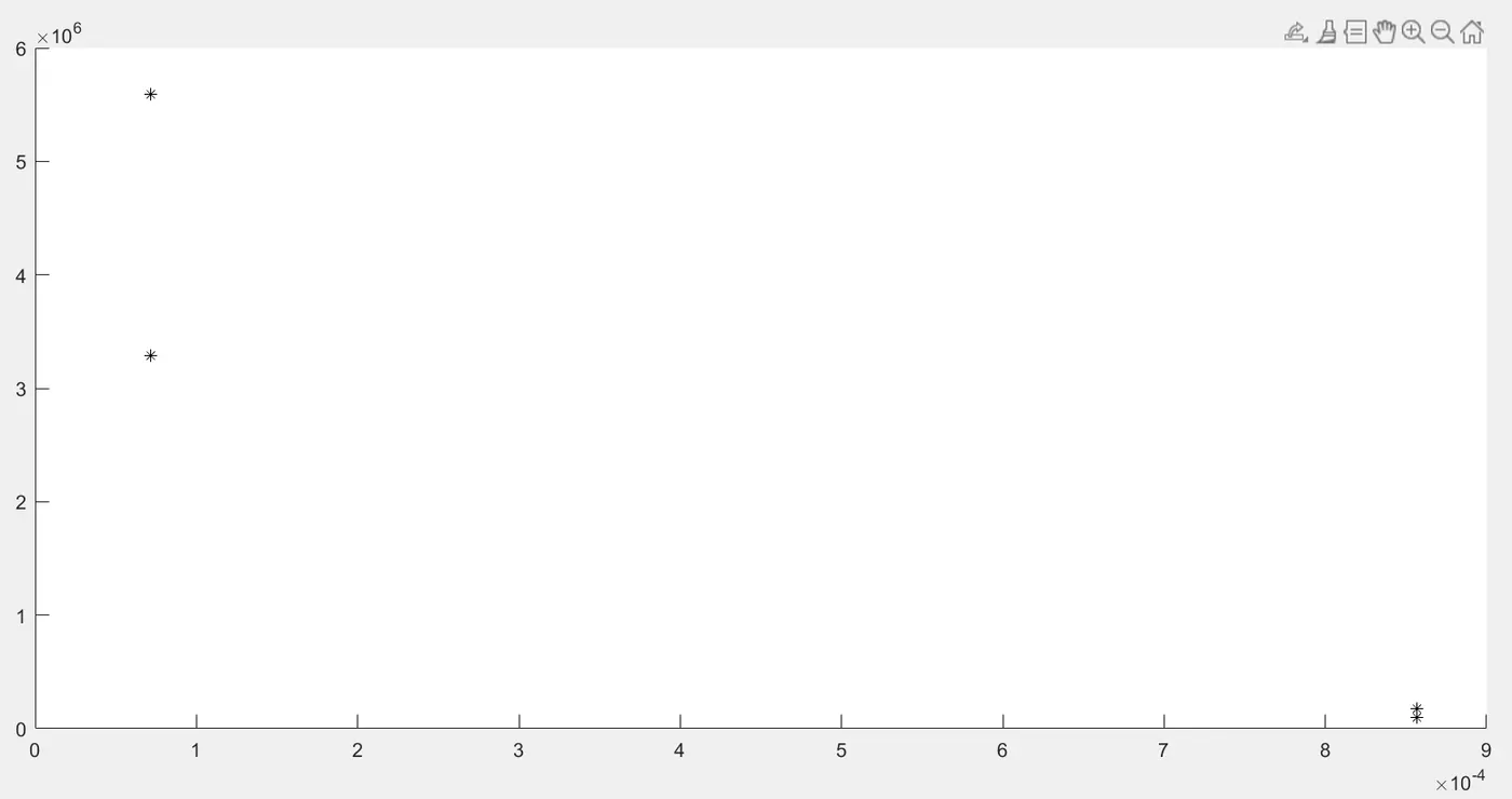
We cannot join these points to form a line because isentropic processes do not have constant slope.If we try,we get the result by using the command which is an error.
plot([v1 v2 v3 v4],[p1 p2 p3 p4],'color','b')
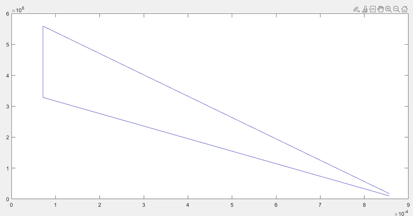
Error elimination:
To plot the diagram correctly, we need two things:
1. Piston kinematics to determinehow the volume changes from top dead centre(TDC) to bottom dead center(BDC) and how does the combustion process volume changes as the function of the crank angle.
2. Thermodynamic relation during compression.
function [V] = engine_kinematics(bore,stroke,cond_rod,cr,start_crank,end_crank)

a = stroke/2;
R = cond_rod/a;

 v_s = pi/4*bore^2*stroke;
 v_c = v_s/(cr-1);

 theta = linspace(start_crank,end_crank,100);

 term1 = 0.5*(cr-1);
 term2 = R +1 - cosd(theta);
 term3 = (R^2 - sind(theta).^2).^0.5;

 V = (1 + term1*(term2 - term3)).*v_c;

end
We need a different formula to calculate how the volume iniside the engine combustion chamber changes.
V/Vc = 1+ 0.5(cr-10)* [ R+1 -cos(angle) — (R² -sin²(angle)⁰.5]
Now we are going to use this program in our first program for getting PV diagram, correctly,but using total program is in-convenient therefore we are introducing the predefined command in MATLAB known as function.
Function [V] =piston_kinematics(bore,stroke,con_rod,cr,start_crank,end_crank)
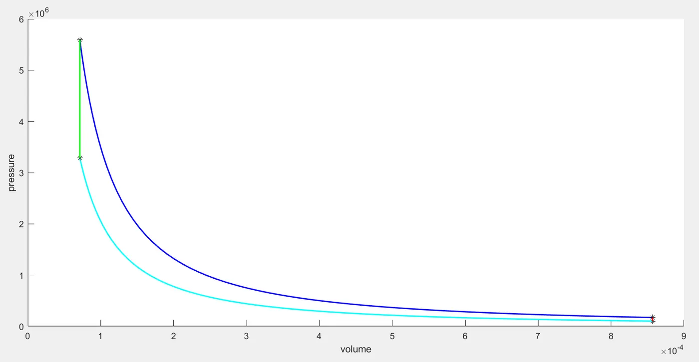
So now in our first program we are going call this function by calling its name.Now we are going to use this function to get the volume and pressure information during the compression and expansion stroke.
 clear all
 close all
 clc

 %Inputs
 gamma = 1.4
 t3 = 2300

 % state variables
 p1 = 101325
 t1 = 500

 %state engine variables
 bore = 0.1;
 stroke = 0.1;
 cond_rod = 0.15;
 cr = 12;

 % calculating the swept volume and the clearence volume
 v_swept = (pi/4)*bore^2*stroke;
 v_clearence = v_swept/(cr-1);

 v1 = v_swept+v_clearence
 v2 = v_clearence

 % state variables at state point 2
 % p1*v1^gamma = p2*v2^gamma
 % p2 = p1*(v1/v2)^gamma
 % p2 = p1*cr^gamma
 p2 = p1*cr^gamma
 % p1v1/t1  = p2v2/t2
 % t2 = p2*v2*t1/(p1*v1)
 t2 = p2*v2*t1/(p1*v1)

 constant_c = p2*v2^gamma
 V_compression = engine_kinematics(bore,stroke,cond_rod,cr,180,0)

 % p_compression*V_compression^gamma = constant_c
 p_compression = constant_c./V_compression.^gamma;
 % state variables at state point 3
 v3 = v2
 % p3v3/t3 = p2v2/t2 | p3 = p2*t3/t2
 p3 = p2*t3/t2

 constant_c = p3*v3^gamma
 V_expansion = engine_kinematics(bore,stroke,cond_rod,cr,0,180)

 % p_expansion*V_expansion^gamma = constant_c
 p_expansion = constant_c./V_expansion.^gamma;
 % state variables at state point 4
 v4 = v1
 % p3v3^gamma = p4v4^gamma  | p4 = p3(v3/v4)^gamma
 p4 = p3*(v3/v4)^gamma

 figure(1)
 hold on
 plot(v1,p1,'*','color','k')
 plot(V_compression,p_compression,'linewidth',1.5,'color','c')
 plot(v2,p2,'*','color','k')
 plot(v3,p3,'*','color','k')
 plot(V_expansion,p_expansion,'linewidth',1.5,'color','b')
 plot(v4,p4,'*','color','k')
 plot([v2 v3],[p2 p3],'linewidth',1.5,'color','g')
 plot([v4 v1],[p4 p1],'linewidth',1.5,'color','r')
 xlabel('volume')
 ylabel('pressure')
To calculate thermal efficiency
Thermal efficiency formula,
Thermal_Efficiency = 1-(1/(cr^(gamma-1)))
 %Thermal efficiency of the engine
 Thermal_efficiency = 1-(1/(cr^(gamma-1)))

 Percentage_Efficiency = (1-(cr^(gamma-1))^-1)*100
The output of thermal and percentage efficiency

ERRORS:
function [V] = engine_kinematics(bore,stroke,cond_rod,cr,start_crank,end_crank)

a = stroke/2;
R = cond_rod/a;

 v_s = pi/4*bore^2*stroke;
 v_c = v_s/(cr-1);

 theta = linspace(start_crank,end_crank,100);

 term1 = 0.5*(cr-1);
 term2 = R +1 - cosd(theta);
 term3 = (R^2 - sind(theta).^2).^0.5;

 Vc = (1 + term1*(term2 - term3)).*v_c;

end
In the above program the output argument V is not mentioned anywhere in the program.

To eliminate this error the output arguments must be declared.
function [V] = engine_kinematics(bore,stroke,cond_rod,cr,start_crank,end_crank)

a = stroke/2;
R = cond_rod/a;

 v_s = pi/4*bore^2*stroke;
 v_c = v_s/(cr-1);

 theta = linspace(start_crank,end_crank,100);

 term1 = 0.5*(cr-1);
 term2 = R +1 - cosd(theta);
 term3 = (R^2 - sind(theta).^2).^0.5;

 V = (1 + term1*(term2 - term3)).*v_c;

end
Now in the above program the output argument V is declared and by calling V_compression the output will be obtained.
Conclusion:
Hence PV diagram is obtained and the thermal efficiency is calculated using matlab.