Ahmed Body Challenge
Simulation of flow over Ahmed body
Aim : To simulate the flow over Ahmed body and determine the Coeffiecient of drag for a velocity of 25 m/s.
Objective(s) : 1. To perform a grid independence test for the simulation.
2. Plot the velocity and pressure contours.
3. Explain the reason for negative pressure in the wake region and significance of separation region.
Therory :
Ahmed body :
The Ahmed body represents a simplified, ground vehicle geometry of a bluff body type. Its shape is simple enough to allow for accurate flow simulation but retains some important practical features relevant to automobile bodies.
Complexly shaped cars are very challenging to model and it’s difficult to quantify the aerodynamic drag computationally.The Ahmed body is a benchmark model widely used in the automotive industry for validating simulation tools.
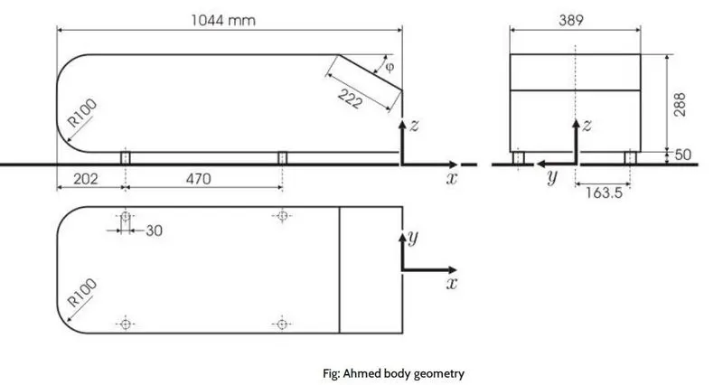
The Ahmed body has a length of 1.044m, heigth of 0.288m and a width of 0.389m. It has 0.5m diameter cylindrical legs attached to the bottom face and the rear surface has a slant of 40 degree.
Necessity for simulating the flow over the Ahmed body :
Aerodynamic drag is one parameter which determines the fuel efficiency of an automobile. The quantification of the aerodynamic drag can be done by the determination of Coefficient of Drag(Cd) or Drag force.
Lower is the drag coefficient, lower is the drag force experienced by the body. Howver, the Coefficient of drag is not a constant. For a particular geometry, the Cd is dependent on Reynolds number, Flow direction, object orientation and surface rougness.
Geometry preparation :
In our case, a STEP file of Ahmed body geometry is imported into the SpaceClaim module. To simplify the computational cost, the symmetry of the geometry is taken advantage of. The geometry is split along the longitudinal plane and only one half of the geometry is considered for simulation.
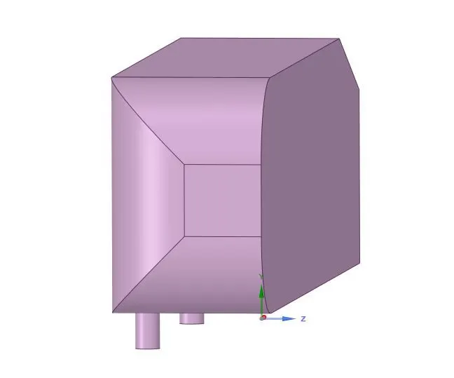
Fig. 2: Truncated model of the Ahmed body
Creation of an enclosure :
A rectangular volume which represents the virtual wind tunnel is created using the "enclosure" option. The dimensions of an enclosure are carefully estimated based on the flow visualized in the experiments. An enclosure which is close to ten times the length of the Ahmed body will effectively contain the flow regime that is observed in the experiments.
In our case the, the enclosure is of the following dimensions: 7m * 1m * 0.5m
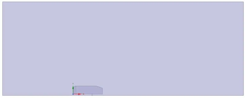
Fig. 3 : Ahmed body enclosed in a virual wind tunnel.
Creation of Mesh :
a. Basic Mesh : The geometry when loaded in the ANSYS Mesher is assigned the boundaries. The extreme left face of the enclosure is named as Inlet and the extreme right face of the enclosure is named as Outlet. The faces of the Ahmed body are collectively named as Car wall.
A good mesh would be the one with the high number of Hexahedral elements as they have the highest orthogonal quality.Second comes the tetra hedral elements. However, it is not always possible to have the Hexahedral elements due to the complex geometry. Also it would require expertise as well time to selectively mesh the computational domain. For this reason we take the advantage of the "Multizone" feature of ANSYS, that generates Hexahedral elements wherever possible.
A basic mesh would look as follows :
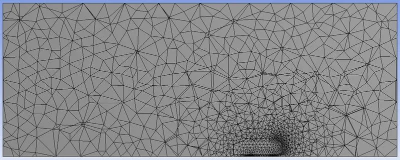
Fig. 4 : Mesh without any refinement zones (Basic mesh)
b. Refined mesh :
Adding a refinement region near to the Ahmed body is a local refinement technique where the mesh close to the geometry is refined rather than refining the mesh in the entire computational domain :
1. Capturing the near wall effects like wake region, flow recirculation and vortices.
2. High accuracy in the results at a lower cell count.
In our case, the local refinement can be done by creating a refinement region inside the enclosure by creating another enclosure but with the reduced size. While there are no fixed measurements for the length, breadth and height of the enclosure, a good estimate is done by observing the velocity contours observed by simulating the basic mesh case. This means the smaller enclosure should be long enough to accomodate wake region/ recirculation zone/ vortices/ near field phenomenon.
In our case an enclosure with the following dimensions is created : 3m (length) * 1m (width) * 0.5m (height).
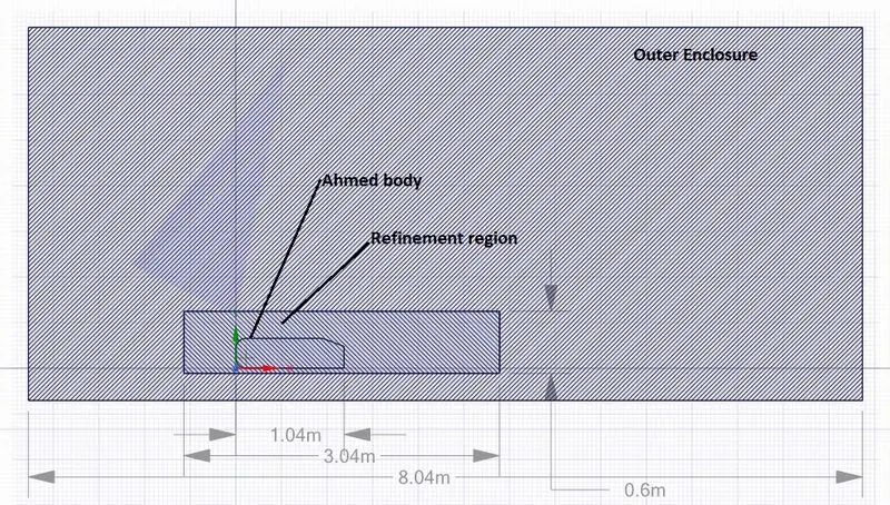
Fig. 5 : Refinement region added to the basic mesh.
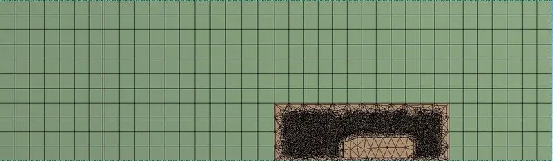
Fig. 6 : A refined mesh with 437,508 cells.
Mesh Metrics :
The X-axis in the chart shows the element quality. 0 being the lowest on the quality scale and 1 being the highest. In our case most of the elements are tetrahedral elements which are above the average in quality.
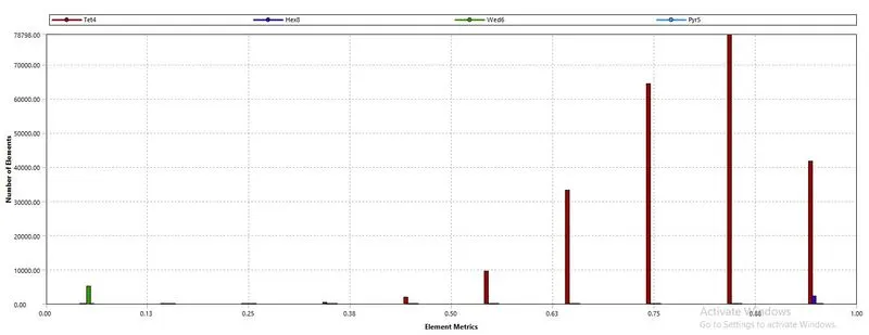
Fig. 7 : Mesh Metrics chart
Case setup in ANSYS Fluent :
The mesh is initially checked for quality as and when it gets loaded in Fluent. Any improvement that is recommended by the console has to be made.
The step by step procedure as shown below has to be followed for succesful case setup :
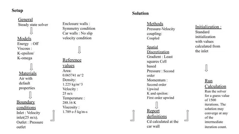
Results :
case.1 : Refined case with 4,37,508 cells
Residual plot:
The solution converged at 278 iterations.
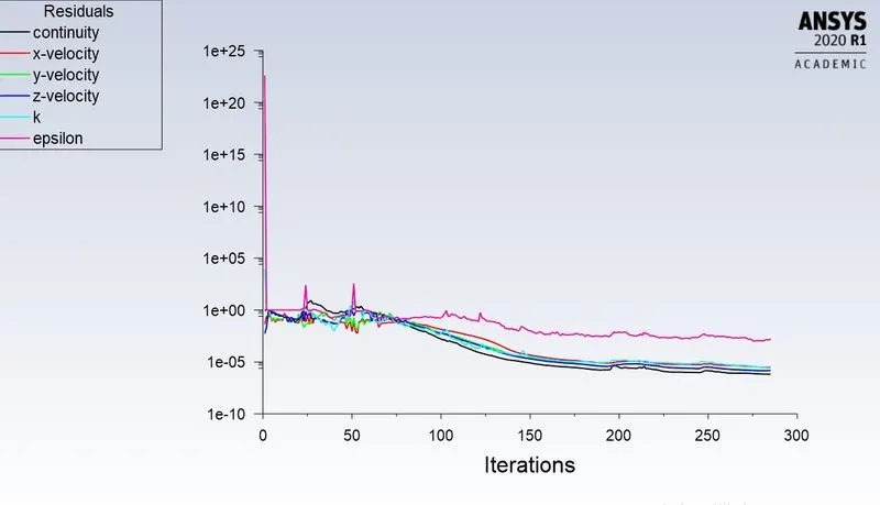
Fig. 8 : Residual plot for N-S equations, K and epsilon showing convergence at 276th step.
Velocity contour :
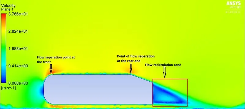
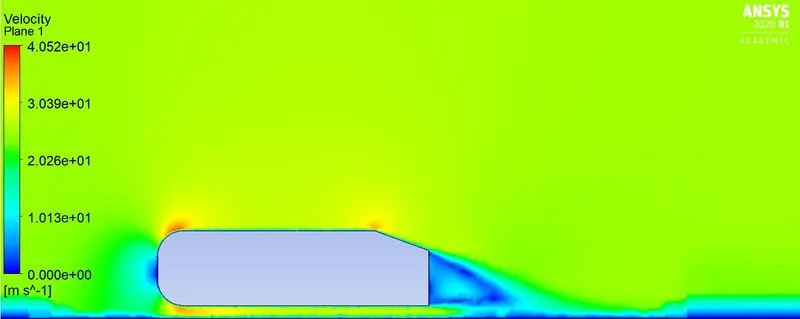
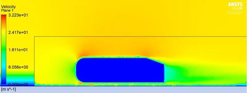
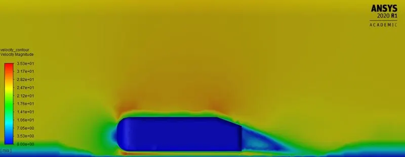
The areas in the orange are unaffected/ least affected by the fluid motion in the other areas. These areas have the velocity which is equivalent to that of the free stream velocity of 25 m/s. Fluid which is in direct contact with the wall of the solid have zero velocity which is because of the No slip velocity condition at the walls.
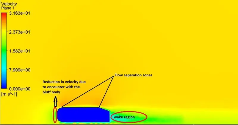
Fig. 9 : Velocity contour plot
Velocity vector plot :
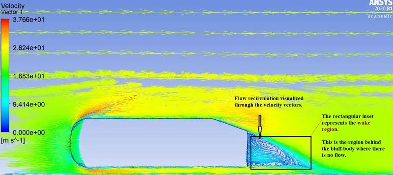
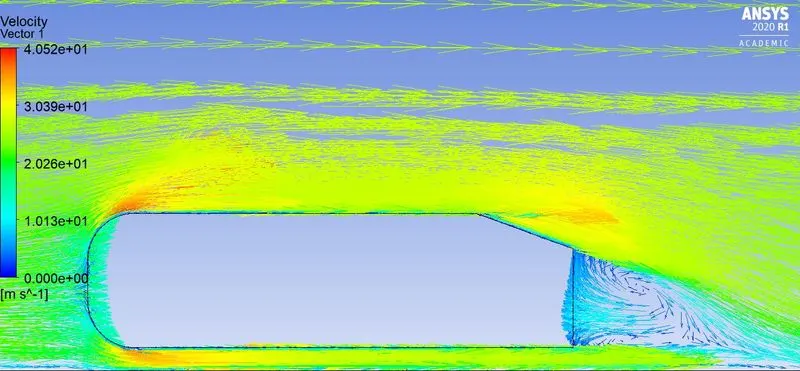
As and when the air which is at freestream velocity (`U_(prop)`) comes in contact with the front of the ahmed body it decelerates and deviates from the original path. It then traces the wall of the body in contact and experiences flow separation because of the adverse pressure gradient.
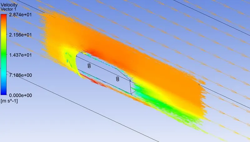
Fig. 10 : Velocity vector plot
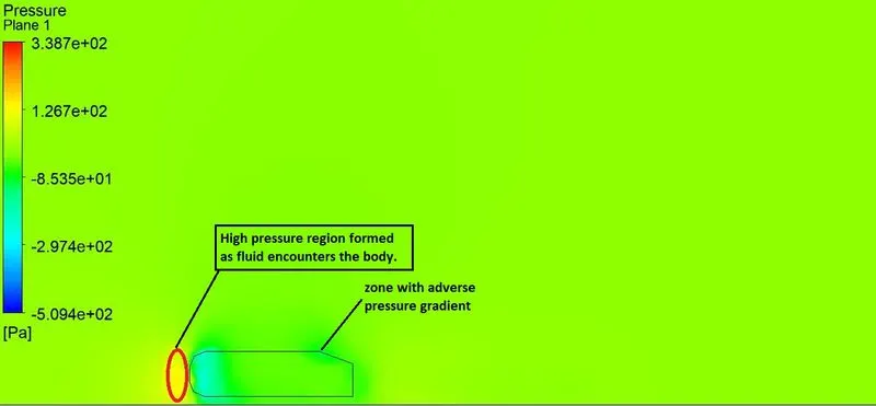
Fig. 11 : Pressure contour plot
Percentage error in calculation of Coefficient of drag :
1. Reference value of the coefficient of drag = 0.33
2. Obtained value of the coefficient of drag = 0.477
% error in the computation = (Difference of the values)/ (Obtained value) *100
= `(0.477 - 0.33)/(0.477)` * 100
= 30.817 %
The error in the computed value is more than 15% and hence it cannot be accepted.
A refinement in the y-plus value can yield a better value of the coefficient of drag.
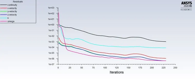
Considering the `K-omega` turbulence model which gives the better resolution of the phenomena occuring at walls - Flow separation, flow reattachment, boundary layer effects and flow recirculation. And for the `K-omega` model to work effectively, a Y-Plus value within 0-5 range is appropriate.
Case.1 : `k-omega`turbulence model with a Y-Plus of 0.1
Mesh details :
Total number of cells : 4,54,872
Residual plot :
Velocity contour plot :
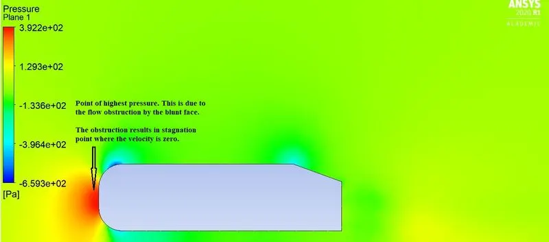
Pressure contour plot :
Velocity vector plot :
Case.2 : `k-omega`turbulence model with a Y-Plus of 0.2
Mesh details :
Total number of cells: 4,18,020
Residual plot :
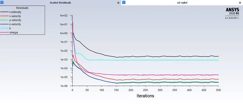
The calculation was performed for 500 iterations and the value of the Coefficient of drag is determined to be 0.2478.
Velocity contour plot :
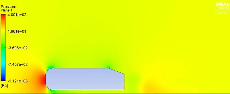
Pressure contour plot :
Velocity vector plot:
Case.3 : `k-omega`turbulence model with a Y-Plus of 0.3
Mesh details:
total number of cells: 4,37,163
Residual plot :
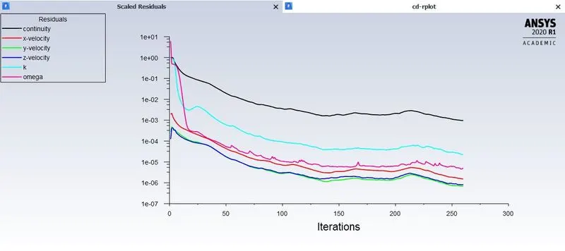
Total number of iterations to converge : 258
Velocity contour plot :
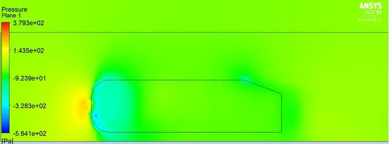
Pressure contour plot :
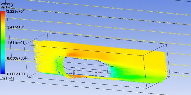
Velocity vector plot :
Case. 4 : `k-omega`turbulence model with a Y-Plus of 0.4
Mesh details :
Cell count : 4,48,868.
Residual plot :
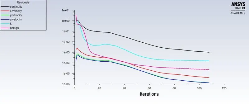
The solution converged at 258 iterations and the Coefficient of drag was determined to be 0.3772.
Velocity contour plot :
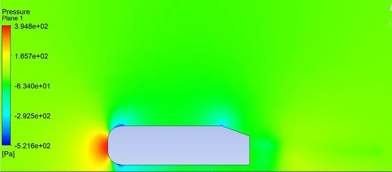
Pressure contour plot:
Velocity vector plot :
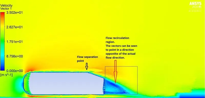
It can be clearly seen that the velocity vectors point in a direction oppsite to that of the actual flow direction. The flow first separates at the front of the body. The second flow separation point lies at the starting point of the slant.
Coefficient of drag plot :
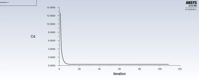
Table of Results for the `k-omega`turbulence model :
| Y-plus value | Number of cells | No. of iterations to converge | Reference Cd value | Coefficient of Drag (Cd) value | % Error |
| 0.1 | 454,872 | 500 (without convergence criteria) | 0.33 | 0.2580 | 21.81 |
| 0.2 | 418,020 | 500 (without convergence criteria) | 0.33 | 0.2478 | 24.90 |
| 0.3 | 437,163 | 258 | 0.33 | 0.3772 | 14.30 |
| 0.4 | 448,868 | 108 | 0.33 | 0.2925 |
11.36 |
Gaps in the simulation :
The Grid independence study hasn't been performed because of the cell count limitation of the ANSYS Student version. However, care was taken in generating the mesh which incorporates the y-plus values which are essential for setting up the inflation layers.
Analysis :
1. Significance of point of separation
Conside the following image which shows the flow of air over a bluff body:
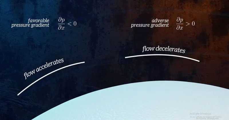
Fig. a : Adverse pressure gradient during the flow over a blunt body [2]
The white region in the above image represents a bluff body (For eg: Ahmed body or cylinder or sphere or any non-streamlined body). When the air passes over the front edge body it accelerates. The flow acceleration results in the increase in velocity of the air and hence decrease in pressure (based on Bernoulli's theorem). This region is called the region of favourable pressure gradient. (`(delp)/(delx) <0`)
But, after travelling a certain distance the flow decelerates which implies decrease in flow velocity. This results in the increase in pressure which is termed as adverse pressure gradient (`(delP)/(delx) > 0`)
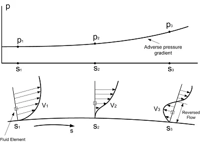
But if the pressure gradient is much larger (`(delP)/(delx) > > 0`), the flow reverses its direction and as it cannot tavel backwards because of the oncoming fluid it detaches from the surface resulting in "Flow separation".
2. Negative pressure in the wake region:
 I
I
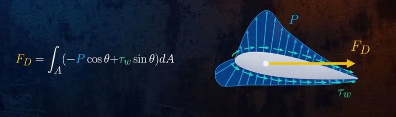
In actuality, the exact value of the Drga forces is calculated by the formula: [3]
`F_D = int(-P*cos(theta) + tau_omega * sin(theta)) dA`
Here,
P represents the dynamic pressure,
`theta`is the angle between the body and the flow.
`tau_w`represents the shear stress acting on the surface.
The first term `-P*cos(theta)` represents the Pressure drag and the second term `tau_w`represents the friction drag.
In the wake region where there is no flow (for practicality, consider the existence of only backward flow). No flow implies that the region is devoid of any air mass .
If we were to apply the the Drag force formula for the wake region it would reduce to `F_D = int(-P*cos(theta)).dA` ------------------(1)
Differentiating the above equation w.r.t A it turns out to be :
`(dF_D)/(dA) = -P.cos(theta)` ---------------------------------------(2)
Rearranging the terms of equation (2) and considering the Dynamic pressure on the L.H.S
`P = -(dF_D)/(dA)*(cos(theta))^-1`
Hence, the Pressure in the wake region is negative.
Resources :
1. Flow separation : https://www.researchgate.net/figure/Pressure-gradient-and-flow-separation_fig1_321641421
2. Flow separation visualization : https://www.youtube.com/watch?v=GMmNKUlXXDs (courtesy of the youtube channel : The Efficient engineer, Understanding aerodynamic drag).
3. Integral equation for drag force : https://physics.stackexchange.com/questions/21404/strict-general-mathematical-definition-of-drag