A MATLAB Program to Solve the steady and unsteady 2D heat conduction problem
AIM: Solving the steady and unsteady 2D heat conduction problem
We need to solve heat conduction problem in steady and unsteady states for 2D.
So, we will start with steady state
1. Steady state analysis
`(del^2T)/(delx^2)+(del^2T)/(dely^2)=0`
Discretizing
`(T_(i-1)-2T_i+T_(i+1))/(Deltax^2) + (T_(j-1)-2T_j+T_(j+1))/(Deltay^2)=0`
`(T_(i-1)+T_(i+1))/(Deltax^2) + (T_(j-1)+T_(j+1))/(Deltay^2)=(2T_i)[1/(Deltax)^2+1/(Deltay)^2]`
`(T_(i-1)+T_(i+1))/(Deltax^2) + (T_(j-1)+T_(j+1))/(Deltay^2)=T_i *k`
`T(i,j)=1/k((T(i-1,j)+T(i+1,j))/dx^2+(T(i,j-1)+T(i,j+1))/dy^2);`
Where,
`k=2[1/(Deltax)^2+1/(Deltay)^2]`
using these equations programming the MATLAB code as follows
A MATLAB Code for 2D steady state heat conduction of a given square domain
Here the matlab code is explained with the help of comments line by line
Inputs are given
Top Boundary = 600 K
Bottom Boundary = 900 K
Left Boundary = 400 K
Right Boundary = 800 K
The following methods are implemented for solving the above euations equations.
1. Jacobi
2. Gauss-seidel
3. Successive over-relaxation
absolute error criteria is 1e-4
clc %clears the command window
clear % clears the workspace
close all % closes all the window

counter=0; %No. of iterations
tol=1e-4; %Tolerance

n_x=10; %No. of grid points on X-axis
n_y=n_x; % No. of grid points on Y-axis

x=linspace(0,1,n_x); %X-co-ordinates
y=x; %Y-co-ordinates
dx=x(2)-x(1); %Distance between two nodes in x -axis
dy=dx;
%Boundary Condition
%Taking loop of boundary conditions to make sure a matrix is created of
%desired value i.e. n_x*n_y and having the boundary conditions
for b=1:2
T(1,:)=600;     %Top Boundary
T(n_x,:)=900;	% Bottom Boundary
T(:,1)=400;     % Left Boundary
T(:,n_y)=800;   % Right Boundary
end

%Taking the value of corner points as an average of the boundaries

T(1,1)=(T(1,2)+T(2,1))/2;
T(1,end)=(T(1,end-1)+T(2,end))/2;
T(end,1)=(T(end-1,1)+T(end,2))/2;
T(end,end)=(T(end,end-1)+T(end-1,end))/2;

% Initial Guess

for i=2:n_x-1
    for j=2:n_y-1
        T(i,j)=298.15;
    end
end
W=1.05; %Relaxation Factor
T_initial=T; %Storing the Intial Value
T_old=T; % Storing the first value
error=1e-2; % Intializing the error
k=2*(1/dx^2+1/dy^2); %CFL

% Taking the input from the user for selecting the iterative method to be
% used
solver=input('Enter the input (1-Jacoboi, 2-SOR Jacobi, 3-Gauss Siedel, 4-SOR GS): ');

while (error>tol)

    for i=2:n_x-1
        for j=2:n_y-1
            if solver==1
%             %Jacobi=Using all the values of previous iteration
            T(i,j)=((T_old(i-1,j)+T_old(i+1,j))/dx^2+(T_old(i,j-1)+T_old(i,j+1))/dy^2)/k;
            elseif solver==2
%             %SOR-Jacobi=Over shooting the values of Jacobi by factor W
            T(i,j)=(1-W)*T_old(i,j)+W*((T_old(i-1,j)+T_old(i+1,j))/dx^2+(T_old(i,j-1)+T_old(i,j+1))/dy^2)/k;
            elseif solver==3
%             %Gauss Siedel=Using values from previous iteration and current iteration if available
            T(i,j)=((T(i-1,j)+T_old(i+1,j))/dx^2+(T(i,j-1)+T_old(i,j+1))/dy^2)/k;
            elseif solver==4
%             %SOR-Gauss Siedel=Over shooting the values of Gauss Siedel by factor W
            T(i,j)=(1-W)*T_old(i,j)+W*((T(i-1,j)+T_old(i+1,j))/dx^2+(T(i,j-1)+T_old(i,j+1))/dy^2)/k;
            else
                fprintf('You have input wrong, Please input again\n');
                solver=input('Enter the input (1-Jacoboi, 2-SOR Jacobi, 3-Gauss Siedel, 4-SOR GS): ');
            end

        end
    end

    error=max(max(abs(T-T_old))); %finding the maximum value in the matrix
    T_old=T; % Replacing the current iteration to previous iteration

    counter=counter+1; %Calculating the no. of iterations

end

        contourf(x,y,T)         %Creates contour with filled colours
        clabel(contourf(x,y,T)) %Labels the temperatures
        colorbar                %Labels the value of colour
        colormap(jet)           %colour pattern
        set(gca, 'ydir' ,'reverse') %Reversing the Y-direction values

        xlabel ('X-Axis') %Labels the X-axis
        ylabel ('Y-Axis') %Labels the Y-axis
        %Writing the title
            if solver==1
             text=sprintf('No. of Jacobi Iterations :%d',counter);
            elseif solver==2
              text=sprintf('No. of SOR-Jacobi Iterations :%d',counter);
            elseif solver==3
              text=sprintf('No. of Gauss Siedel Iterations :%d',counter);
            elseif solver==4
              text=sprintf('No. of SOR-Gauss Siedel Iterations :%d',counter);
            end

        title(text)    %Labels the title
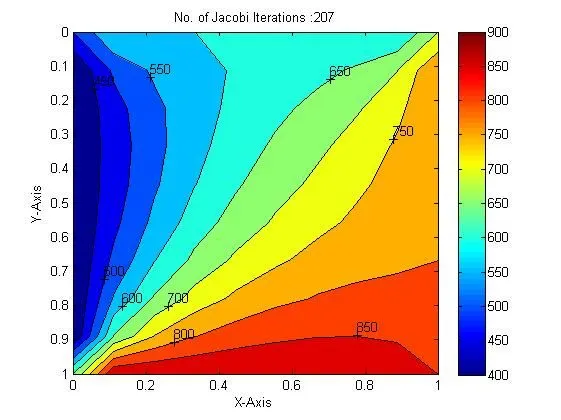
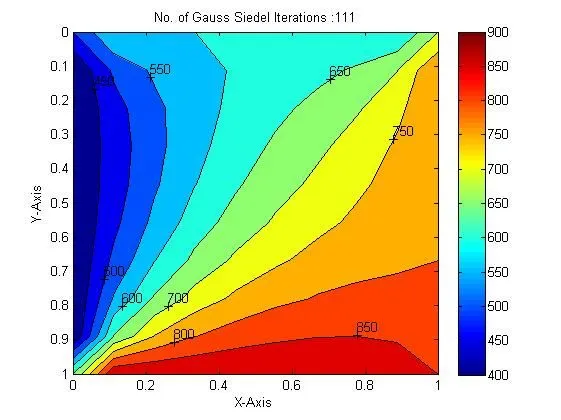
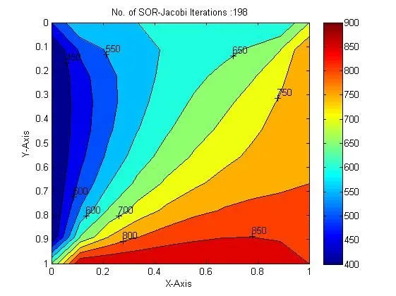
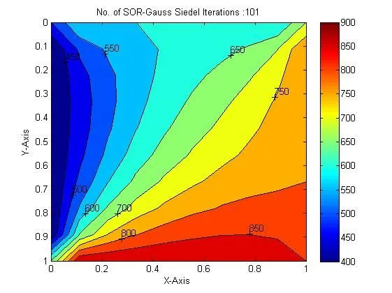
So, lets list out no. of iterations for each method
1. Jacobi = 207
2. Gauss-seidel =111
3. Successive over-relaxation - Jacobi = 198
4. Successive over-relaxation - Gauss-seidel = 101
So, from the above obtained data we can conclude that
Jacobi Iterations>Gauss-Seidel Iterations>SOR Iterations
2. Transient state analysis
`(delT)/(delt)=alpha[(del^2T)/(delx^2)+(del^2T)/(dely^2)]`
`alpha = "Thermal Diffusivity"`
Discretizing
`(T_i^(n+1)-T_i^n)/(Deltat)=alpha[(T_(i-1)-2T_i+T_(i+1))/(Deltax^2) + (T_(j-1)-2T_j+T_(j+1))/(Deltay^2)]^(n or n+1)`
as we are taking spatial derivative so it does not matter if we take n or n+1
if we take it as n the solution is called as explicit solution
here all the terms on right side are known at n time step
`(T_i^(n+1)-T_i^n)/(Deltat)=alpha[(T_(i-1)-2T_i+T_(i+1))/(Deltax^2) + (T_(j-1)-2T_j+T_(j+1))/(Deltay^2)]^n`
`T_i^(n+1)=[T_i+k_1(T_(i-1)-2T_i+T_(i+1)) + k_2(T_(j-1)-2T_j+T_(j+1))]^n`
where,
These are also known as CFL numbers
`k_1=alpha(Deltat)/(Deltax^2) =CFL_x`
`k_2=alpha(Deltat)/(Deltay^2) =CFL_y`
`CFL <=0.5`
which means
`CFL_x+CFL_y <=0.5`
If CFL>0.5 solution becomes unstable
Here,
`alpha=1.5`
`dt=1e-3`
`dx=dy=1/9`
so, `CFL_x+CFL_y =2*(1.5*(1e-3))/(1/9)^2`
`CFL_x+CFL_y =0.2430<0.5`
so, the solution is stable
A MATLAB Code for 2D unsteady state heat conduction of a given square domain solving explicitly
Here the matlab code is explained with the help of comments line by line
Inputs are given
Top Boundary = 600 K
Bottom Boundary = 900 K
Left Boundary = 400 K
Right Boundary = 800 K
absolute error criteria is 1e-4
here we are not using any iterative methods because all the terms on the present time step that is n is known and we are finding for next time step
clc %clears the command window
clear %clears the workspace
close all

counter=0; %Iterations count
tol=1e-4; %tolerance

n_x=10; %No. of nodes on x axis
n_y=n_x; % No. of nodes on y axis

x=linspace(0,1,n_x); %X-co-ordinates
y=x;%Y-co-ordinates
dx=x(2)-x(1); %Distance between two nodes in x -axis
dy=dx;        %Distance between two nodes in y -axis

%Boundary Condition

%Taking loop of boundary conditions to make sure a matrix is created of
%desired value i.e. n_x*n_y and having the boundary conditions
for b=1:2
    T(1,:)=600;   %Top Boundary
    T(n_x,:)=900; % Bottom Boundary
    T(:,1)=400;   % Left Boundary
    T(:,n_y)=800; % Right Boundary
end
%Corner Points value by taking average
T(1,1)=(T(1,2)+T(2,1))/2;
T(1,end)=(T(1,end-1)+T(2,end))/2;
T(end,1)=(T(end-1,1)+T(end,2))/2;
T(end,end)=(T(end,end-1)+T(end-1,end))/2;

% Initial Guess

for i=2:n_x-1
    for j=2:n_y-1
        T(i,j)=298.15;
    end
end


T_initial=T;
error=1e-2; %error term
time=0; %Intializing the time

alpha =1.5; %thermal diffusivity
dt=1e-3; % time step
k_1=alpha*dt/dx^2; %CFLx
k_2=alpha*dt/dy^2; %CFLy

h = figure;
axis tight manual % this ensures that getframe() returns a consistent size
filename = 'explicit_transient.gif';


for nt=1:150 %time loop
    T_prev=T; %updating the values for new time step
    error=1e-2; %reassigning the error to operate the loop
while (error>tol) %space loop
        T_old=T; %updating the values for next iteration
    for i=2:n_x-1 % starting from 2 & ending from end-1
        for j=2:n_y-1 %because boundary conditions are fixed
            T(i,j)=(T_prev(i,j)+k_1*(T_prev(i-1,j)-2*T_prev(i,j)+T_prev(i+1,j))+k_2*(T_prev(i,j-1)-2*T_prev(i,j)+T_prev(i,j+1)));
        end
    end

    error=max(max(abs(T-T_old))); %finding the max error in matrix
    counter=counter+1; %counting the iterations
end
time=time+1; %counting the time step

        contourf(x,y,T)         %Creates contour with filled colours
        clabel(contourf(x,y,T)) %Labels the temperatures
        colorbar                %Labels the value of colour
        colormap(jet)
        set(gca, 'ydir' ,'reverse') %Reversing the Y-direction values

        xlabel ('X-Axis') %Labels the X-axis
        ylabel ('Y-Axis') %Labels the Y-axis
        text=sprintf('No. of time steps :%d',time);
        title(text)    %Labels the title
        pause(0.03);      %Pause the graph

        %GENERATING GIF

         drawnow
      % Capture the plot as an image
      frame = getframe(h);
      im = frame2im(frame); % To get image data from a single movie frame
      [imind,cm] = rgb2ind(im,256); %To convert RGB data to indexed image data
      % imind=image_data %im=indexed_image %cm=color_map
      % Write to the GIF File
      if nt == 1
          imwrite(imind,cm,filename,'gif', 'Loopcount',inf,'DelayTime',0.3);
      else
          imwrite(imind,cm,filename,'gif','WriteMode','append','DelayTime',0.3);
          % To append multiple images to first image
      end
end 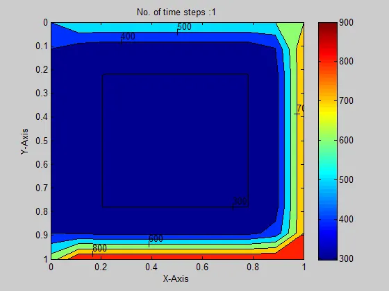
Here as we can see from the plot how heat is been transmitted and after around 150 time steps we can gey steady state solution we can increase the time step to increase the accuracy but after certain point it becomes meaningless to move ahead because the change in temperature will be neligible.
IMPLICIT METHOD
Rewritng the above dicretized equation for unsteady state heat conduction in 2D again
`(T_i^(n+1)-T_i^n)/(Deltat)=alpha[(T_(i-1)-2T_i+T_(i+1))/(Deltax^2) + (T_(j-1)-2T_j+T_(j+1))/(Deltay^2)]^(n or n+1)`
if we take it as n+1 the solution is called as implicit solution
here all the terms on right side are unknown at n+1 time step
`(T_i^(n+1)-T_i^n)/(Deltat)=alpha[(T_(i-1)-2T_i+T_(i+1))/(Deltax^2) + (T_(j-1)-2T_j+T_(j+1))/(Deltay^2)]^(n+1)`
`T_i^(n+1)=T_i^n+[alpha*(Deltat)/(Deltax^2)*(T_(i-1)-2T_i+T_(i+1)) + alpha*(Deltat)/(Deltay^2)(T_(j-1)-2T_j+T_(j+1))]^(n+1)`
`T_i^(n+1)=T_i^n+k_1*(T_(i-1)-2T_i+T_(i+1))^(n+1) + k_2(T_(j-1)-2T_j+T_(j+1))^(n+1)`
Where,
`k_1=alpha*(Deltat)/(Deltax^2)`
`k_2=alpha*(Deltat)/(Deltay^2)`
`T_i^(n+1)=T_i^n+k_1T_(i-1)^(n+1)-2k_1T_i^(n+1)+k_1T_(i+1)^(n+1) + k_2T_(j-1)^(n+1)-2k_2T_j^(n+1)+k_2T_(j+1)^(n+1)`
`T_i^(n+1)+2k_1T_i^(n+1)+2k_2T_j^(n+1)=T_i^n+k_1T_(i-1)^(n+1)+k_1T_(i+1)^(n+1) + k_2T_(j-1)^(n+1)+k_2T_(j+1)^(n+1)`
`T^(n+1)(1+2k_1+2k_2)=T_i^n+k_1(T_(i-1)+T_(i+1))^(n+1) + k_2(T_(j-1)+T_(j+1))^(n+1)`
`T^(n+1)=1/(1+2k_1+2k_2)*[T_i^n+k_1(T_(i-1)+T_(i+1))^(n+1) + k_2(T_(j-1)+T_(j+1))^(n+1)]`
`T^(n+1)=1/(1+2k_1+2k_2)T_i^n+k_1/(1+2k_1+2k_2)(T_(i-1)+T_(i+1))^(n+1) + k_2/(1+2k_1+2k_2)(T_(j-1)+T_(j+1))^(n+1)]`
`T^(n+1)=term1*T_i^n+term2*(T_(i-1)+T_(i+1))^(n+1) + term3*(T_(j-1)+T_(j+1))^(n+1)`
`term1=1/(1+2k_1+2k_2)`
term2=k_1*term1=k_1/(1+2k_1+2k_2)
term3=k_2*term1=k_2/(1+2k_1+2k_2)
`T^(n+1)=term1*T_i^n+term2*(T_(i-1)+T_(i+1))^(n+1) + term3*(T_(j-1)+T_(j+1))^(n+1)`
A MATLAB Code for 2D unsteady state heat conduction of a given square domain solving implicitly
Here the matlab code is explained with the help of comments line by line
Inputs are given
Top Boundary = 600 K
Bottom Boundary = 900 K
Left Boundary = 400 K
Right Boundary = 800 K
The following methods are implemented for solving the above euations equations.
1. Jacobi
2. Gauss-seidel
3. Successive over-relaxation
absolute error criteria is 1e-4
clc %clears the command window
clear %clears the workspace
close all

counter=0; %Iterations count
tol=1e-4; %tolerance

n_x=10; %No. of nodes on x axis
n_y=n_x; % No. of nodes on y axis

x=linspace(0,1,n_x); %X-co-ordinates
y=x;%Y-co-ordinates
dx=x(2)-x(1); %Distance between two nodes in x -axis
dy=dx;        %Distance between two nodes in y -axis

%Boundary Condition
%Taking loop of boundary conditions to make sure a matrix is created of
%desired value i.e. n_x*n_y and having the boundary conditions

for b=1:2
    T(1,:)=600;   %Top Boundary
    T(n_x,:)=900; % Bottom Boundary
    T(:,1)=400;   % Left Boundary
    T(:,n_y)=800; % Right Boundary
end
%Corner Points value by taking average
T(1,1)=(T(1,2)+T(2,1))/2;
T(1,end)=(T(1,end-1)+T(2,end))/2;
T(end,1)=(T(end-1,1)+T(end,2))/2;
T(end,end)=(T(end,end-1)+T(end-1,end))/2;

% Initial Guess

for i=2:n_x-1
    for j=2:n_y-1
        T(i,j)=298.15;
    end
end

W=1.1; %SOR factor
T_initial=T;

error=1e-2; %error term

time=0; %Intializing the time
alpha =1; %thermal diffusivity
dt=1e-3; % time step
k_1=alpha*dt/dx^2;
k_2=alpha*dt/dy^2;

%Asking the iterative technique from the user
solver=input('Enter the input (1-Jacoboi, 2-Gauss Siedel, 3-SOR Jacobi 4-SOR GS): ');

h = figure;
axis tight manual % this ensures that getframe() returns a consistent size
filename = 'implicit_transient.gif';


for nt=1:150 %time loop
    T_prev=T; %updating the values for new time step
    while (error>tol) %space loop
            T_old=T; %updating the values for next iteration
        for i=2:n_x-1 % starting from 2 & ending from end-1
            for j=2:n_y-1 %because boundary conditions are fixed
                %splitting the equations in terms to minimize the
                %complexity of the equation

                term1=(1+2*k_1+2*k_2)^-1;
                term2=k_1*term1;
                term3=k_2*term1;
                %selcting the iterative technique
                if solver==1
                solver_name='Jacobi Method';
                T(i,j)=term1*T_prev(i,j)+term2*(T_old(i-1,j)+T_old(i+1,j)) + term3*(T_old(i,j-1)+T_old(i,j+1));

                elseif solver==2
                solver_name='Gauss Siedel';
                T(i,j)=term1*T_prev(i,j)+term2*(T(i-1,j)+T_old(i+1,j)) + term3*(T(i,j-1)+T_old(i,j+1));

                elseif solver==3
                solver_name='Successive OR Relaxation (SOR)-Jacobi';
                T(i,j)=((1-W)*T_old(i,j))+W*(term1*T_prev(i,j)+term2*(T_old(i-1,j)+T_old(i+1,j)) + term3*(T_old(i,j-1)+T_old(i,j+1)));

                elseif solver==4
                solver_name='Successive OR Relaxation (SOR)-Gauss Siedel';
                T(i,j)=((1-W)*T_old(i,j))+W*(term1*T_prev(i,j)+term2*(T(i-1,j)+T_old(i+1,j)) + term3*(T(i,j-1)+T_old(i,j+1)));

                else
                fprintf('You have input wrong, Please input again\n');
                solver=input('Enter the input (1-Jacoboi, 2-Gauss Siedel, 3-SOR Jacobi, 4-SOR GS): ');
                end
            end
        end

        error=max(max(abs(T-T_old))); %finding the max error in matrix
        counter=counter+1; %counting the iterations
    end
time=time+1; %counting the time step
error=1e-2; %reassigning the error to operate the loop
%counter=0; % reassining the iteration to zero for clculating the iteration

        contourf(x,y,T)         %Creates contour with filled colours
        clabel(contourf(x,y,T)) %Labels the temperatures
        colorbar                %Labels the value of colour
        colormap(jet)
        set(gca, 'ydir' ,'reverse') %Reversing the Y-direction values

        xlabel ('X-Axis') %Labels the X-axis
        ylabel ('Y-Axis') %Labels the Y-axis
        text=sprintf('No. of time steps in %s is :%d',solver_name,time);
        title(text)    %Labels the title
        pause(0.00003);      %Pause the graph

         %GENERATING GIF

         drawnow
      % Capture the plot as an image
      frame = getframe(h);
      im = frame2im(frame); % To get image data from a single movie frame
      [imind,cm] = rgb2ind(im,256); %To convert RGB data to indexed image data
      % imind=image_data %im=indexed_image %cm=color_map
      % Write to the GIF File
      if nt == 1
          imwrite(imind,cm,filename,'gif', 'Loopcount',inf,'DelayTime',0.3);
      else
          imwrite(imind,cm,filename,'gif','WriteMode','append','DelayTime',0.3);
          % To append multiple images to first image
      end

end
counter
OUTPUT:
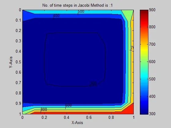
Enter the input (1-Jacoboi, 2-Gauss Siedel, 3-SOR Jacobi 4-SOR GS): 1
counter =
1239
OUTPUT:
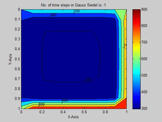
Enter the input (1-Jacoboi, 2-Gauss Siedel, 3-SOR Jacobi 4-SOR GS): 2
counter =
979
OUTPUT:
Enter the input (1-Jacoboi, 2-Gauss Siedel, 3-SOR Jacobi 4-SOR GS): 3
counter =
1024
OUTPUT:
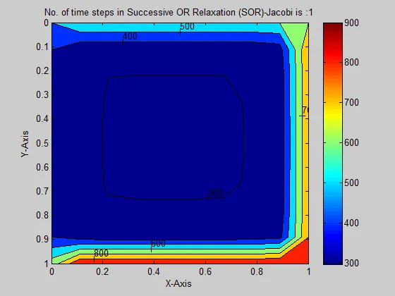
Enter the input (1-Jacoboi, 2-Gauss Siedel, 3-SOR Jacobi 4-SOR GS): 4
counter =
841
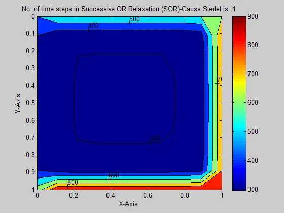
So, lets list out no. of iterations for each method for 150 time steps
1. Jacobi = 1239
2. Gauss-seidel = 979
3. Successive over-relaxation - Jacobi = 1024
4. Successive over-relaxation - Gauss-seidel = 841
So, from the above obtained data we can conclude that
Jacobi Iterations>Gauss-Seidel Iterations>SOR Iterations
So, from the above obtained plots we can conclude that
Jacobi Iterations>Gauss-Seidel Iterations>SOR Iterations
Here as we can see from the plot how heat is been transmitted and after around 150 time steps we can gey steady state solution we can increase the time step to increase the accuracy but after certain point it becomes meaningless to move ahead because the change in temperature will be neligible.