A MATLAB Program to Find Effect of Varying Timesteps for Linear Convection

Effect of time step size on the solution

A function file that accepts the time step as an argument and solves the linear convection problem.

DATA :

1. Number of nodes, n = 80

2. Time step , dt = 1e-4, 1e-3, 1e-2, and 1e-1

3. Simulation run time , t = 0.4 seconds.

The MATLAB code is explained with the help of comments mentioned in the code to understand code line by line

Inputs in function file is time step and color while output are velocity, initial velocity and node distance

outputs are chosen to plot original data

% A Function file that accepts the time step as an argument and solves the
%linear convection problem. 

function [u, uinitial,x] = time_stamp(dt,color)
    
    % Inputs
    L=1; %[m] % Domain Length
    n=80; % Number of Nodes
    x=linspace(0,L,n); % Node
    dx=x(2)-x(1); % Grid Size
    c=1; %[m/s] %Constant convection coefficient
    t=0.4; %[s] % Simulation run time
    
    % Step function

    for i=1:length(x)
        if x(i)>=0.1 && x(i)<=0.3
            u(i)=2;%[m/s]
        else
            u(i)=1;%[m/s]
        end
    end

    uold=u;
    uinitial=u;
    %time loop
    for k = 1:t/dt
        %space loop
        for i=2:n
            u(i)=uold(i)-c*dt*(uold(i)-uold(i-1))/dx;
        end
        uold=u; % Transmitting the values for next time step
    end
        hold on 
        
        plot(x,u,color)     % Plots the graph
        axis([0 L 0 2])     % Limits the axis
        xlabel('x')         % Labels the X-axis
        ylabel('Velocity')  % Labels the Y-axis
end

MATLAB Program to call the function file and generate plots

%Effect of time step size on the solution

clc % clears the COmmand Window
clear % clears the Workspace
close all % closes the  window

% Inputs for the function
dt=[1e-4,1e-3,1e-2,1e-1]; % Varying Time step
color=['c','y','m','k']; % Varying color code for time step

%Color Codes
%c = cyan
%y = yellow
%m = magenta
%k = black

for z=1:4
   %outputs=function(inputs) 
   [u(z,:),uinitial,x]= time_stamp(dt(z),color(z));   
  
end

%outputs are retrived to plot intial data
plot(x,uinitial,'b') % Initial Graph
legend('1e-4','1e-3','1e-2','1e-1','data')
%To differentiate all the plots

OUTPUT:

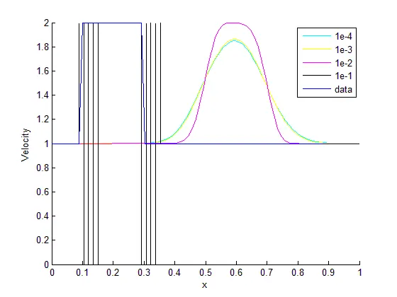
Change in time tep size affects numerical diffusion, instability, the courant number and accuracy.

As we can see from the above graph that change in time step can effect stability of the system as we know that courant number depends on time step so change in it above certain value can lead to instability keeping other terms constant.

The above graph also depicts that change in time step may also lead into decreasing velocity this may occur due to error term which we may have neglected this error term is similar to the diffusing term in Navier Stoke's equation therefore error term we can call as artificial diffusion or numerical diffusion so change in time step size also effects the accuracy in the system.

CFL criteria that govern the linear convection equation.

The Courant–Friedrichs–Lewy or CFL condition is a condition for the stability of unstable numerical methods that model convection or wave phenomena. As such, it plays an important role in CFD

It follows that for any explicit simple linear convection problem, the Courant number must be equal or smaller than 1: `C<=1`

Courant Number , C = c dt/dx = c dt/(L/(n-1))

Calculating Courant Number for varying time stamps

dt=1e-4 C = 1*1e-4/(1/(80-1)) = 0.0079

dt=1e-3 C = 1*1e-3/(1/(80-1)) = 0.079

dt=1e-2 C = 1*1e-2/(1/(80-1)) = 0.79

dt=1e-1 C = 1*1e-1/(1/(80-1)) = 7.9 >1

Criteria application on implicit solution

Implicit (matrix) solvers are usually less sensitive to numerical instability and so larger values of Cmax may be tolerated. So, it does not apply on implicit solution.