A MATLAB Program to derive 4th order approximation of a 2nd order derivative using Taylor Table method

Deriving 4th order approximations of the second-order derivative.

1. Central difference

`(del^2u)/(dx^2)=af(i-2)+bf(i-1)+cf(i)+df(i+1)+ef(i+2)`

	f(x)	`Deltaxf'(x)`	`Deltax^2f''(x)`	`Deltax^3f'''(x)`	`Deltax^4f''''(x)`
af(i-2)	1a	-2a	2a	-4a/3	2a/3
bf(i-1)	1b	-1b	b/2	-1b/6	1b/24
cf(i)	1c	0	0	0	0
df(i+1)	1d	1d	d/2	1d/6	1d/24
ef(i+2)	1e	2e	2e	4e/3	2e/3
Total	0	0	1	0	0

Equations:

`a+b+c+d+e=0`

`-2a-b+d+2e=0`

`2a+b/2+d/2+2e=1`

`-4a/3-b/6+d/6+4e/3=0`

`2a/3+b/24+d/24+2e/3=0`

Solving These Equations we will get the value of constants

a= -0.0833 = -1/12
b= 1.3333 = 16/12
c= -2.5000 = -30/12
d= 1.3333 = 16/12
e= -0.0833 =-1/12

`(del^2u)/(dx^2)=af(i-2)+bf(i-1)+cf(i)+df(i+1)+ef(i+2)=(2a+b/2+d/2+2e)Deltax^2f''(x)+O(Deltax^6)`

Dividing by `Deltax^2`we get

`(af(i-2)+bf(i-1)+cf(i)+df(i+1)+ef(i+2))/(Deltax^2)=(1)f''(x)+O(Deltax^4)`

So, here we are neglecting terms to the power four so it is upto 4th order approximate

The order of accuracy P = Number of nodes in the stencil N - order of derivative Q + 1 for symmetric/central schemes

Here, N=5, Q=2, Scheme=1

P=5-2+1

P=4

`f''(x)=(-f(i-2)+16f(i-1)-30f(i)+16f(i+1)-f(i+2))/(12Deltax^2)`

2. Skewed right-sided difference

`(del^2u)/(dx^2)=af(i)+bf(i+1)+cf(i+2)+df(i+3)+ef(i+4)+gf(i+5)`

	f(x)	`Deltaxf'(x)`	`Deltax^2f''(x)`	`Deltax^3f'''(x)`	`Deltax^4f''''(x)`	`Deltax^5f'''''(x)`
af(i)	1a	0	0	0	0	0
bf(i+1)	1b	b	b/2	b/6	b/24	b/120
cf(i+2)	1c	2 c	2c	4c/3	2c/3	4c/15
df(i+3)	1d	3 d	9d/2	9d/2	27d/8	81d/40
ef(i+4)	1e	4 e	8e	32e/3	32e/3	128e/15
gf(i+5)	1g	5g	25g/2	125g/6	625g/24	625g/24
Total	0	0	1	0	0	0

Equations:

`a+b+c+d+e+g=0`

`b+2c+3d+4e+5g=0`

`b/2+2c+9d/2+8e+25g/2=1`

`b/6+4c/3+9d/2+32e/3+125g/6=0`

`b/24+2c/3+27d/8+32e/3+625g/24=0`

`b/120+4c/15+81d/40+128e/15+625g/24=0`

Solving These Equations we will get the value of constants

a= 3.7500
b= -12.8333
c= 17.8333
d= -13.0000
e= 5.0833
g= -0.8333

`(del^2u)/(dx^2)=af(i)+bf(i+1)+cf(i+2)+df(i+3)+ef(i+4)+gf(i+5)=(1)Deltax^2f''(x)+O(Deltax^6)`

Dividing by `Deltax^2`we get

`(af(i)+bf(i+1)+cf(i+2)+df(i+3)+ef(i+4)+gf(i+5))/(Deltax^2)=(1)f''(x)+O(Deltax^4)`

So, here we are neglecting terms to the power four so it is upto 4th order approximate

The order of accuracy P = Number of nodes in the stencil N - order of derivative Q + 0 for one-sided/skewed schemes

Here, N=6, Q=2, Scheme=0

P=6-2+0

P=4

`f''(x)=(45f(i)-154f(i+1)+214f(i+2)-156f(i+3)+61f(i+4)-10f(i+5))/(12Deltax^2)`

3. Skewed left-sided difference

`(del^2u)/(dx^2)=af(i)+bf(i-1)+cf(i-2)+df(i-3)+ef(i-4)+gf(i-5)`

++++	f(x)	`Deltaxf'(x)`	`Deltax^2f''(x)`	`Deltax^3f'''(x)`	`Deltax^4f''''(x)`	`Deltax^5f'''''(x)`
af(i)	1a	0	0	0	0	0
bf(i-1)	1b	-1b	b/2	-1b/6	1b/24	-1b/120
cf(i-2)	1c	-2c	2c	-10c/3	2c/3	-4c/15
df(i-3)	1d	-3d	9d/2	-9d/2	27d/8	-81d/40
ef(i-4)	1e	-4e	8e	-32e/3	32e/3	-128e/15
gf(i-5)	1g	-5g	25g/2	-125g/6	625g/24	-625g/24
Total	0	0	1	0	0	0

Equations:

`a+b+c+d+e+g=0`

`-b-2c-3d-4e-5g=0`

`b/2+2c+9d/2+8e+25g/2=1`

`-b/6-10c/3-9d/2-32e/3-125g/6=0`

`b/24+2c/3+27d/8+32e/3+625g/24=0`

`-b/120-4c/15-81d/40-128e/15-625g/24=0`

Solving These Equations we will get the value of constants

a= 3.7500
b= -12.8333
c= 17.8333
d= -13.0000
e= 5.0833
g= -0.8333

`(del^2u)/(dx^2)=af(i)+bf(i-1)+cf(i-2)+df(i-3)+ef(i-4)+gf(i-5)=(1)Deltax^2f''(x)+O(Deltax^6)`

Dividing by `Deltax^2`we get

`(af(i)+bf(i-1)+cf(i-2)+df(i-3)+ef(i-4)+gf(i-5))/(Deltax^2)=(1)f''(x)+O(Deltax^4)`

So, here we are neglecting terms to the power four so it is upto 4th order approximate

The order of accuracy P = Number of nodes in the stencil N - order of derivative Q + 0 for one-sided/skewed schemes

Here, N=6, Q=2, Scheme=0

P=6-2+0

P=4

`f''(x)=(45f(i)-154f(i-1)+214f(i-2)-156f(i-3)+61f(i-4)-10f(i-5))/(12Deltax^2)`

A program in Matlab to evaluate the second-order derivative of the analytical function exp(x)*cos(x) & Comparing it with the 3 numerical approximations that have been derived above.

Creating a function file for 4th order approximation for second derivative

%Creating a function file for 4th order approximation for second 
%derivative

function ffx=central_difference(x,dx)
% Creating the Taylor Table
for i=0:4
    for j=0:4
        if i<3
            taylor_table_3(i+1,j+1)=(-1)^j*((2-i)^j)/(factorial(j));
        else
            taylor_table_3(i+1,j+1)=((i-2)^j)/(factorial(j));
        end
    end
end
% Finding the constants
A_3= taylor_table_3'^-1*[0;0;1;0;0];

cds=0;
for i=1:5
    fx(i)=exp(x+(i-3)*dx)*cos(x+(i-3)*dx);
    cds=A_3(i)*fx(i)+cds;
end

%Second order Derivative
ffx=cds/(dx)^2;

end

Creating a function file for 4th order approximation for second derivative skewed left

%Creating a function file for 4th order approximation for second 
%derivative skewed left

function ffslx=skewed_left(x,dx)
%output=function(Inputs)

%Creating a taylor table
for i=0:5
    for j=0:5
        taylor_table_2(i+1,j+1)=(-1)^j*(i^j)/(factorial(j));    
    end
end
% getting the constants
A_2= inv(taylor_table_2')*[0;0;1;0;0;0];


bds=0;
for i=1:6
   
    bds=bds+A_2(i)*exp(x+(1-i)*dx)*cos(x+(1-i)*dx);
  
end

ffslx=bds/(dx)^2;
%Second Derivative for skewed left
end

Creating a function file for 4th order approximation for second derivative skewed right

%Creating a function file for 4th order approximation for second 
%derivative skewed right


function ffsrx=skewed_right(x,dx)

% Creating the Taylor Table
for i=0:5
    for j=0:5
        taylor_table(i+1,j+1)=(i^j)/(factorial(j));    
    end
end

A_1= (taylor_table'^-1)*[0;0;1;0;0;0];

fds=0;
for i=1:6
    fds=fds+A_1(i)*exp(x+(i-1)*dx)*cos(x+(i-1)*dx);
end

ffsrx=fds/(dx)^2;
%Second Derivative for skewed right
end

A MATLAB Program to derive 4th order approximation of a 2nd order derivative using Taylor Table method

% A MATLAB Program to derive 4th order approximation of a 2nd order 
% derivative using Taylor Table method

clc % clears the command window
clear %clears the workspace
close all % closes other matlab windows

% Inputs
x=pi;%/3;
dx=linspace(pi/2,pi/10,200); %range



% Analytical Method
f_x=exp(x)*cos(x); % Main Function
% f1x=-exp(x)*sin(x)+cos(x)*exp(x); %First Derivative
f2x= -2*exp(x)*sin(x); % Second Derivative


for i=1:length(dx)
    ffx=central_difference(x,dx(i));
    error1(i)=abs(f2x-ffx);
    ffsrx=skewed_right(x,dx(i));
    error2(i)=abs(f2x-ffsrx);
    ffslx=skewed_left(x,dx(i));
    error3(i)=abs(f2x-ffslx);
end

loglog(dx,error1,'r')
hold on
loglog(dx,error2,'g')
loglog(dx,error3,'b')
xlabel('dx')
ylabel('error')
legend('Central Difference','Skewed Right','Skewed Left')

A plot that compares the absolute error between the above-mentioned schemes

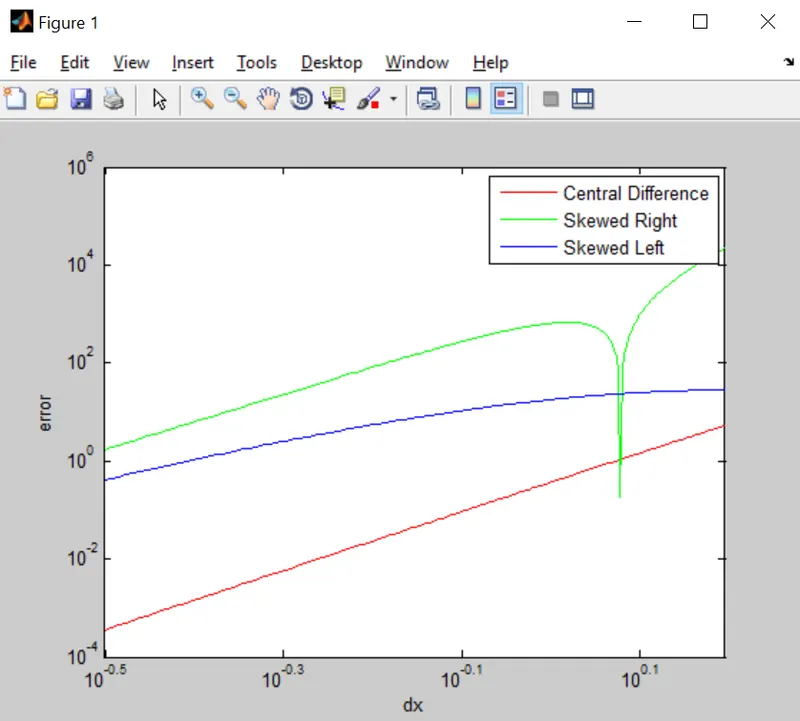
As we can observe from the plot that the error for the central scheme is very low while for the left skewed scheme and right skewed scheme is almost similar but much higher than central

We can also observe that as thw value of dx decreases the error reduces

A skewed scheme is useful & can do that a CD scheme cannot

A skewed scheme is useful because at certain times it may be possible that we will not have data from any of the directions so in that case a skewed scheme is more useful.

A CD scheme cannot calculate values at end boundary points which a skewed scheme can