A MATLAB Program of Numerical solution to the One-dimensional Linear Convection equation

Numerical solution to the One-dimensional Linear Convection equation.

Given Data:

1. Domain length is L = 1m

2. The initial velocity profile is a step function (t=0)

v(x = 0.1 to 0.3) = 2m/s

v(x=0 to 0.1 & x = 0.3 to 1) = 1m/s

3. Constant convection coefficient, c = 1 m/s

4. Time step, dt = 0.01

5. Simulation run time , t = 0.4 seconds.

1D Linear convection equation

`(delu)/(delt)+c(delu)/(delx)=0`

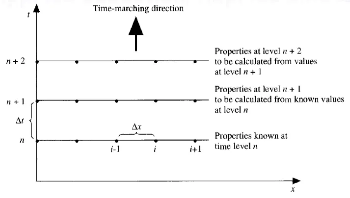
Discretizing the equation using first-order forward differencing for the time derivative and using first-order backward/rearward differencing for the space term.

`(u_k^(n+1)-u_k^n)/(Deltat)+c[(u_k^n-u_(k-1)^n)/(Deltax)]=0`

`u_k^(n+1)=u_k^n+c (Deltat)/(Deltax) [(u_k^n-u_(k-1)^n)]`

Finding the velocity at k node at n+1 time step with the help of above formula

A MATLAB Program for simulation for varying Number of nodes, n=20,40,80 and 160.

-The program is explained with the help of comments in the program

clc % clears the command window
clear % clears the workspace
close all

L=1; %[m] % Domain Length
n=160; % no. of nodes
x=linspace(0,L,n); % Node points
dx=x(2)-x(1); % grid size
c=1; %[m/s] %Constant convection coefficient
t=0.4; %[s] % Simulation run time
dt=0.01; %Time step



% Step function

for i=1:length(x)
    if x(i)>=0.1 && x(i)<=0.3
        u(i)=2;%[m/s]
    else
        u(i)=1;%[m/s]
    end
end


% time derivative - forward approximation
% space derivative - backward approximation
%du=-cdt du/dx - Governing Equation

h = figure;
axis tight manual % this ensures that getframe() returns a consistent size
filename = 'Convection_Animated.gif';

plot(x,u,'red','LineWidth',2)
xlabel('x')
ylabel('velocity')

uold=u;
uintial=u;
for k = 1:n*t
    for i=2:n
        u(i)=uold(i)-c*dt*(uold(i)-uold(i-1))/dx;
    end
    uold=u; %intial velocity
    hold on % prevents rewriting of the image
    plot(x,u) % plots the figure
    axis([0 L 1 2]) %Specifying the limits
       
    pause(0.3) % pausing the plot to visualize the image movement
    
    drawnow 
      % Capture the plot as an image 
      frame = getframe(h); 
      im = frame2im(frame); % To get image data from a single movie frame 
      [imind,cm] = rgb2ind(im,256); %To convert RGB data to indexed image data
      % imind=image_data %im=indexed_image %cm=color_map
      % Write to the GIF File 
      if k == 1 
          imwrite(imind,cm,filename,'gif', 'Loopcount',inf,'DelayTime',0.3); 
      else 
          imwrite(imind,cm,filename,'gif','WriteMode','append','DelayTime',0.3);
          % To append multiple images to first image
      end 
end

Output:

n=20

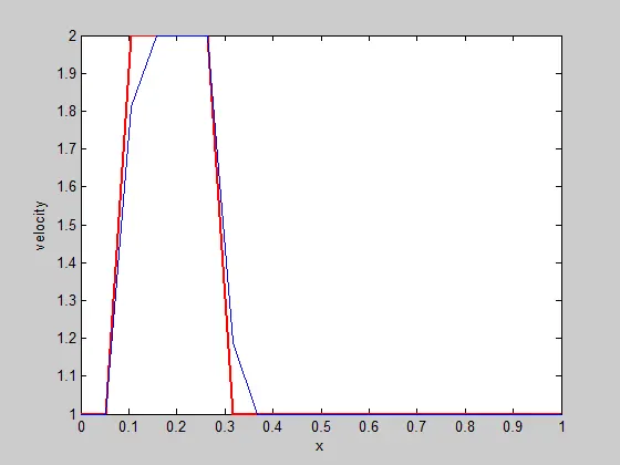
n=40

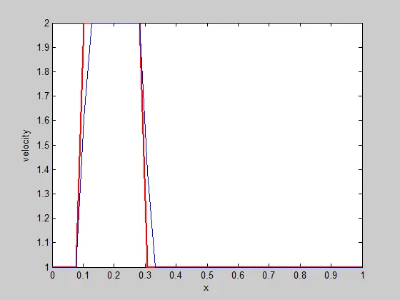
n=80

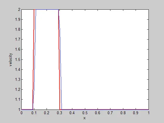
n=160

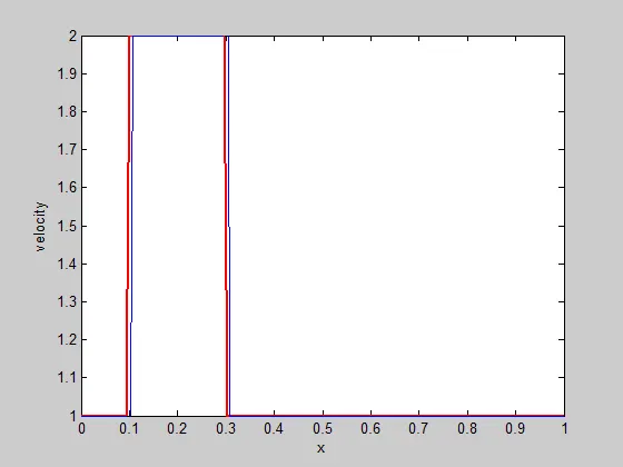
From the plots obtained we observe

(1) Numerical diffusion

While n=20 as the wave is moving its peak velocity is decreasing in the sense diffusing is taking place but it is not implemented in the equation so, it is the error term which we have neglected which is similar with the diffusion term of navier stokes equation, that error term we can call as artificial diffusion or numerical diffusion

So, by increasing the no. of nodes we can minimize this error but up to certain limit to keep the system stable which is discussed below

(2) Instability

The Courant–Friedrichs–Lewy or CFL condition is a condition for the stability of unstable numerical methods that model convection or wave phenomena. As such, it plays an important role in CFD

It follows that for any explicit simple linear convection problem, the Courant number must be equal or smaller than 1: `C<=1`

Courant Number , C = c dt/dx = c dt/(L/(n-1))

Calculating Courant Number for various nodes

n=20 C = 1*0.01/(1/(20-1)) = 0.19

n=40 C = 1*0.01/(1/(40-1)) = 0.39

n=80 C = 1*0.01/(1/(80-1)) = 0.79

n=160 C = 1*0.01/(1/(160-1)) = 1.59 >1

so change in grid size can effect accuracy and stability of the solution so, we need to find the limiting value of grid size to keep system in stable condition and also increase the no. of nodes to improve accuracy.