Write a code to fit a linear and cubic polynomial data for given cp data .

Aim- Write a program to code a curve fit both linear and cubic polynomial for given cp data.

THEORY -

CURVE FITTING :

It is the process of construct a curve or mathematical functions,which passes the closest oriximity to the real series of data .By curve fitting ,we can mathematically construct the functional relationship between the observed data set and parameter values .It is a highly effective in the mathematically modify of some natural process.

Assume data points (x1,y1),(x2,y2),.......(xn,yn) and assume the best fit fir set of these points with be y = f(x) under which the equation of the curve will be the best is possible as follows

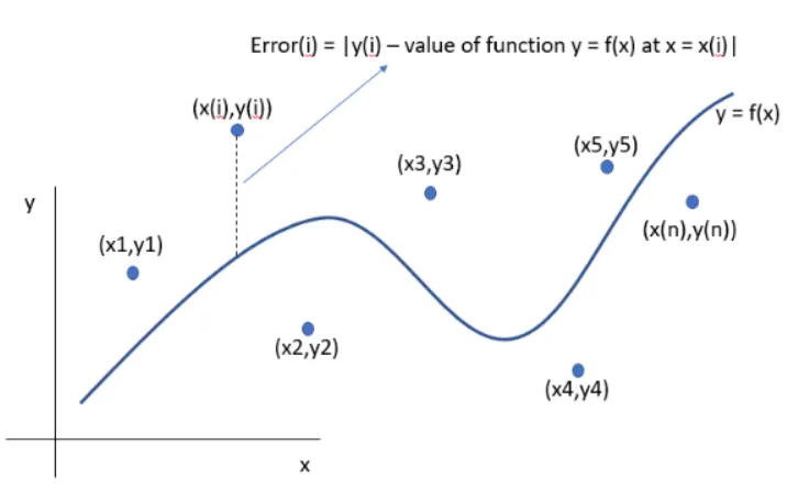
How to choose it is best fit

there are four thing on which best curve fit depens there are :-

1 sum of square due to error (SSE)

2 R - square .

3 Adjusted R - square .

4 Root mean square error( RMSE)

if R-square value is between 0.9500 to 1.000 the curve is consider as a best fit .

R-SQUARE :

it is a quantity that measure how successfully the fit is explaining the variation of data ,when it seems the higher the value of R-square is better fit and lower it is bad fit .

R- square ranges a value 0 to 1 .

The value of R-square can be calculated by using formula .

R^2 = SSR/SST

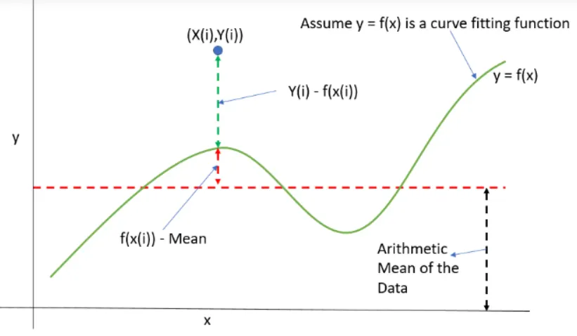
IF y = f(x) is the fit curve then SSR is defined as follows

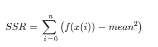
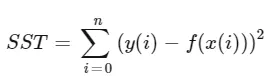
SST = SSR+SSE

From above we get

R^2 = SSR/SST

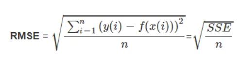
where 'n' is total jno of data points available

MATLAB CODE FOR BOTH LINEAR AND CUBIC POLYNOMIAL WITHOUT SPLITTING:

clear all
close all
clc
%preparing the data

cp_data = load('data')

temperature = cp_data(:,1);
cp = cp_data(:,2);

% curve fit

%cp = a*T^2+b*T+c

coeffs = polyfit(temperature,cp,2);
predicted_cp = polyval(coeffs,temperature);
% of linear curve
coeffs1 = polyfit(temperature,cp,1);
predicted_cp1 = polyval(coeffs1,temperature);

% of cubic curve
coeffs2 =polyfit(temperature,cp,3);
predicted_cp2 = polyval(coeffs2,temperature);



% plotting

plot(temperature,cp,'linewidth',3,'color','b');

hold on
plot( temperature,predicted_cp1,'linewidth',3,'color','g');
plot( temperature,predicted_cp2,'linewidth',3,'color','r');
xlabel('temperature [k]')
ylabel('specific heat[ kj/mol-k]')

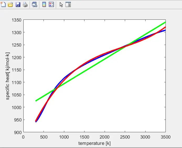
otput graph for this-

MATLAB CODE FOR BOTH LINEAR AND CUBIC POLYNOMIAL WITH SPLITING AND FINDING THE BEST CURVE :

clear all
close all
clc

% preparing the data

cp_data = load('data')
temperature  = cp_data(:,1);

cp = cp_data(:,2);
x = mean(cp)

n = 8

% linear curve fit 
coeffs1 = polyfit(temperature,cp,1);

predicted_cp1 = polyval(coeffs1,temperature);
% split
a = 1;
b = 3200/n

for j= 1:n
    
    coeffs1_split = polyfit(temperature(a:b),cp(a:b),1);
    predicted_cp1_split(a:b) = polyval(coeffs1_split,temperature(a:b));
    a = b+1;
    b =b +3200/n
    
end
plot(temperature,cp,'linewidth',5)

hold on

plot(temperature,predicted_cp1_split,'linewidth',5,'color','r')

% calculation R square  for linear fit for the split

SSR1 = 0;
SSE1 = 0;

for i  = 1:length(cp)/n
    SSR1 = SSR1+ (predicted_cp1_split(i)-x).^2;
    SSE1 = SSE1+ (cp(i)-predicted_cp1_split(i)).^2;
    Rsquare1 = SSR1/(SSR1 + SSE1)
    RMSE1 = (SSE1/length(cp)).^0.5
end


xlabel('temperature[k]')
ylabel('specific heat [KJ/Kmol-K]')


% cubic curve fit
coeffs2 = polyfit(temperature,cp,3);
predicted_cp2 = polyval(coeffs2,temperature);

% split
a =1
b = 3200/n
for j = 1:n
    coeffs2_split = polyfit(temperature(a:b),cp(a:b),3);
predicted_cp2_split(a:b) = polyval(coeffs2_split,temperature(a:b));

a = b+1
b = b+3200/n
end

plot(temperature,predicted_cp2_split,'linewidth',3,'color','g')

% calculation R square  for cubic fit for the split

SSR2 = 0;
SSE2 = 0;

for    i = 1: length(cp)/n
    SSR2 = SSR2 + (predicted_cp2_split(i)-x).^2;
    SSE2 = SSE2+(cp(i)-predicted_cp2_split(i)).^2;
    Rsquare2 = SSR2/(SSR2+SSE2)
    RMSE2 = (SSE2/length(cp)).^0.5
end
xlabel('temperature[k]')
ylabel('specific heat[Kj/mol-k]');
legend('original dataset','linear curve fit','cubic curve fit')

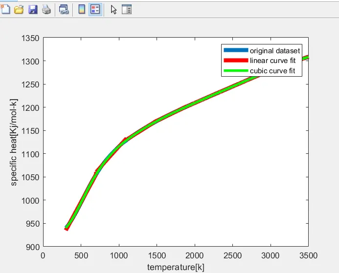
OUTGRAPH FOR THIS :

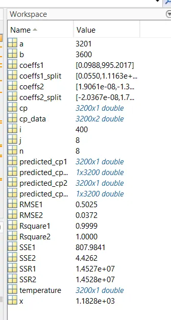
WORSPACE RESULTS :

CONCLUSION :

As we can see from workspace result that the value of Rsquare lies between the 0.9500 to 1 which is suitable range for best fit curves .Hence we can say that the obtained curved is the best fit curve for this given data .