Week 9 - Senstivity Analysis Assignment

Senstivity Analysis Assignment

Objective:

The main aim of this challenge is to extarct the top 10 most sensitivity reactions from the GRI mechanism which is affected with respect to temperature. Plotting the sensitivities for the reactions extarcted.

THEORY:

SENSITIVITY ANALYSIS:

In previous challenges we have learned about the Ignition delay and the factors which affect the ignition dealy which are Temperature, Pressure and the fuel composition. We know that in any reaction mechanism, there will be an inovlement of elementary reactions, the rate of these reaction effects the entire reaction mechanism. The rate of reactions are completely depends on the temperature, pressure and the fuel composition. If we change any of these parameters, the entire reaction rates will be effected. So the change in the ouput depends on the input parameters is caluculated by performing Sensitivity analysis. Suppose p is the parameter and the consider output as y, the change of y is depends in the change of p.

`Sensitivity = dy/(dp)`

Sensitivity analysis becomes very important now a days, as to reeduce the Nox emissions, these days we are using EGR techniques and even for HCCI engines, the input temperature, pressure and the fuel compostion will vary. If we came to know, the combustion is sensitive to particular parameter, the chemists will tune those parameters to reduce the ignition delay.

CODE SNIPPET:

"""
Performing Sensitivity analysis on Methane Combustion.
The fuel mixture consudering is stoichometric

Extracting the top 10 Temperature sensitive reactions

"""

import sys
import cantera as ct 
import numpy as np 
import matplotlib.pyplot as plt 

#Creating a gas object using solution class
gas = ct.Solution('gri30.xml')
temp = 1500
pres = ct.one_atm
#Setting the conditions for the gas object to initialise the combustion
gas.TPX = temp,pres,'CH4: 1, O2: 2 , N2:7.52'
#Creating the reactor as per the given problem
r = ct.IdealGasConstPressureReactor(gas)
#Creating a Reactor network to connect the reactors
sim = ct.ReactorNet([r])

#Extracting the reaction data of methane as per GRI 3.0
reactions = gas.reaction_equations()
n = gas.n_reactions

#Adding all the reactions to the sensitivity mechanism
for i in range(n):
	r.add_sensitivity_reaction(i)

#Setting the tolerance values for ODE of all species 
sim.rtol = 1e-6
sim.atol = 1e-15

#Setting the tolerance values for ODE of sensivity equation
sim.rtol_sensitivity = 1e-6
sim.atol_sensitivity = 1e-6

#Creating an array to store the sensitivity values of all reactions
sT_max = [0]*n

#Creating state array object to store all the values of property of each reactor 
states = ct.SolutionArray(gas,extra = ['t_ms','t'])
#Creating an array to number the reactions of gas object
reac_num = np.arange(1,n+1)


#Initialising the reactor by time and integrating 

for t in np.arange(0,2e-3,5e-6):
	sim.advance(t)
	states.append(r.thermo.state,t_ms = t*1e3, t =t)

	for j in range(n):
		sT = sim.sensitivity('temperature',j)

		if abs(sT) >= abs(sT_max[j]):
			sT_max[j]= sT

			

s_abs = np.abs(sT_max)


#Sorting and zipping the data to extract top reactions and sensitivies

reactions = [a for b, a in sorted(zip(s_abs,reactions),reverse =True)]
react_num = [a for b, a in sorted(zip(s_abs,reac_num),reverse = True)]
sT_max = [a for b, a in sorted(zip(s_abs,sT_max), reverse = True)]

#Slicing the top 10 reactions for zipped data
N = 10

Reactions = reactions[0:N]
Reaction_ID = react_num[0:N]
Sensitivity = sT_max[0:N]

#Creating the table to Print the Sensitivity Values of Reactions
from prettytable import PrettyTable as PT
x = Reaction_ID
y = Reactions
z = Sensitivity

table = PT(['Reaction_ID', 'Reactions', 'Sensitivity'])
for i in range(N):
	table.add_row([x[i],y[i],z[i]])

print('Top 10 Most Sensitive Reactions:') 
print(table)

#PLotting time (vs) temperature
plt.figure(1)
plt.subplot(2, 2, 1)
plt.plot(states.t_ms, states.T)
plt.xlabel('Time (ms)')
plt.ylabel('Temperature (K)')
plt.title('Plot showing the Temperature againist Time')
#Plotting time (vs) 'OH' concentration
plt.subplot(2, 2, 2)
plt.plot(states.t_ms, states('OH').X)
plt.xlabel('Time (ms)')
plt.ylabel('OH Mole Fraction')
plt.title('Plot showing the OH concentration againist Time')
#Plotting time (vs) 'H' concentration
plt.subplot(2, 2, 3)
plt.plot(states.t_ms, states('H').X)
plt.xlabel('Time (ms)')
plt.ylabel('H Mole Fraction')
plt.title('Plot showing the H concentration againist Time')
#Plotting time (vs) 'CH4' concentration
plt.subplot(2, 2, 4)
plt.plot(states.t_ms, states('CH4').X)
plt.xlabel('Time (ms)')
plt.ylabel('CH4 Mole Fraction')
plt.tight_layout()
plt.title('Plot showing the CH4 concentration againist Time')



#Plotting the Top 10 Reaction sensitivities 
plt.figure(2)
plt.barh(Reactions, Sensitivity, 0.4, color= 'black')
plt.xlabel('Sensitivity')
plt.ylabel('Reactions')
plt.title('Top 10 most Sensitive Reactions with respect to Temperature of GRI Mechanism 3.0')
plt.gca().invert_yaxis()
plt.grid()
plt.tight_layout()
plt.show()

PROCEDURE:

• Importing all the necessary modules to python like cantera, numpy, matplotlib and sys.
• Initilaising by creating a gas instance from a Solution class of GRI 3.0 mechanism.
• Setting up the initial conditions using gas.TPX method available in cantera and setting temperature as 1500k, pressure as 1 bar and the species concentration as CH4 of 1 mole, O2 of 2 moles and N2 of 7.52 moles.
• Creating a instance r of Ideal gas constant pressure reactor and a instance sim of reactor network.
• Extracting all the reaction equations involved in methane combustion as per GRI 3.0 mechanism.
• Adding all these equations to the sensitivity reaction by add_sensitivity_reaction method.
• Setting up the realtive and absolute tolerance values for both the reaction ODE's and Sensitivity ODE.
• Creating a states object of SolutionArray class to store all the parameters data for each timestep.
• Using Sim.advance method integrating the system with a time step of 5e-6 for a simulation time of 2e-3.
• Appending all the states by using .append method.
• Inside the same time loop for all the reactions caluculating the sensitivity by using .sensitivity method with respect to temperature and the species.
• After extarcting maximum sensitivity for all reactions, sorting and zipping the data from higher to lower order.
• After sorting, slicing the data for upto 10 reactions.
• Creating a table by usnig Pretty table maodule.
• Plotting the graphs as per the given requirement.

RESULTS:

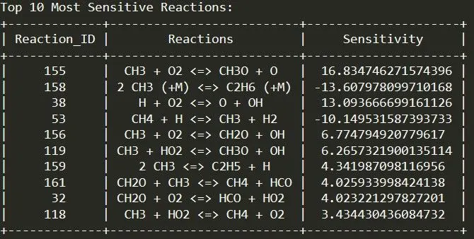
As per the given challenge, the top most 10 sensitive reactions with respect to temperatue is shown in the below table in a decreasing order.

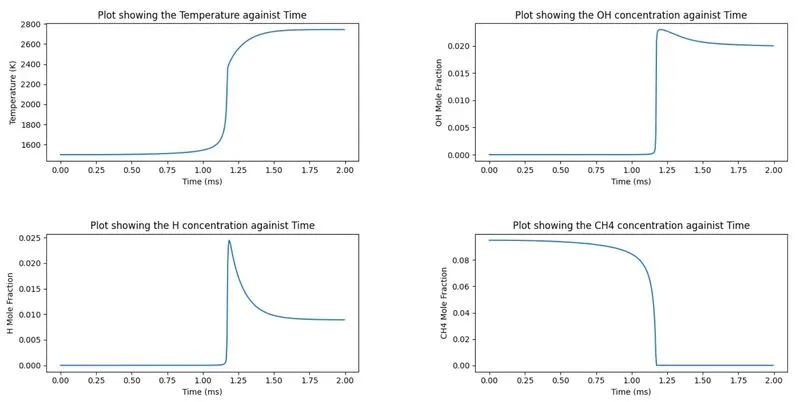
Plot showing the temperature and species concentration change with respect to time:

OBSERVATION:

• By observing the above plots, it makes sense as the temperature remains almost constant equal to initial temperature upto 1 ms and after the iginition takes place, it raises immediately and reaches adiabatic flame temperaturte after sometime.
• By looking the OH plot, it is aso remains zero for some time and raises immediately. It is an important radicle to initiate the ignition.
• By looking the CH4 plot, the concentration is almost equal to 1 at initial stage and simulation takes place drops which makes sense.

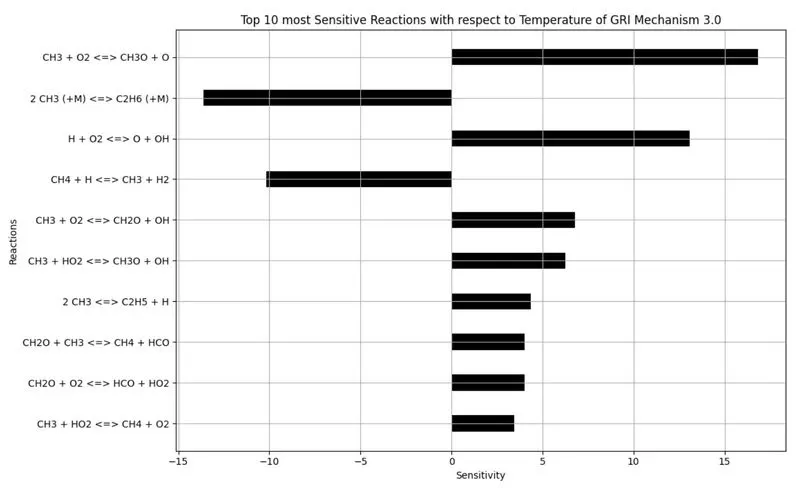
A graph of sensitivities vs the reactions as shown in the sensitivity theory video:

• 

OBSERVATION:

The positive sensivity tells us the increase in the initial temperature will increase the rate of reaction of those reactions and the negative sensitivity is of decrease the reaction rate. If the reactions need to takes place rapidly, by tuning the positive sensitive parameters to increase the reaction rates.