Week 9 - Parametric study on Gate valve.
Aim:- We have to perform a parametric study on the gate valve simulation by setting the opening from 10 % to 80%.
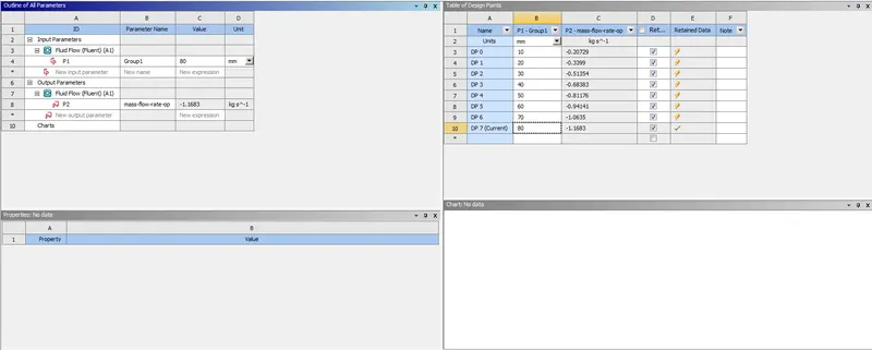
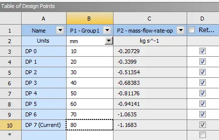
- Obtain the mass flow rates at the outlet for each design point.
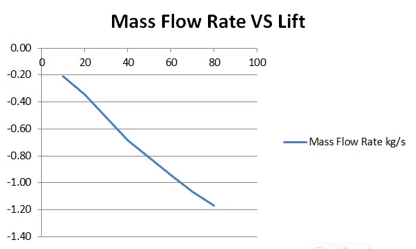
- Calculate the flow coefficient and flow factor for each opening and plot the graph.
- Discuss the results of the mass flow rate and flow coefficient.
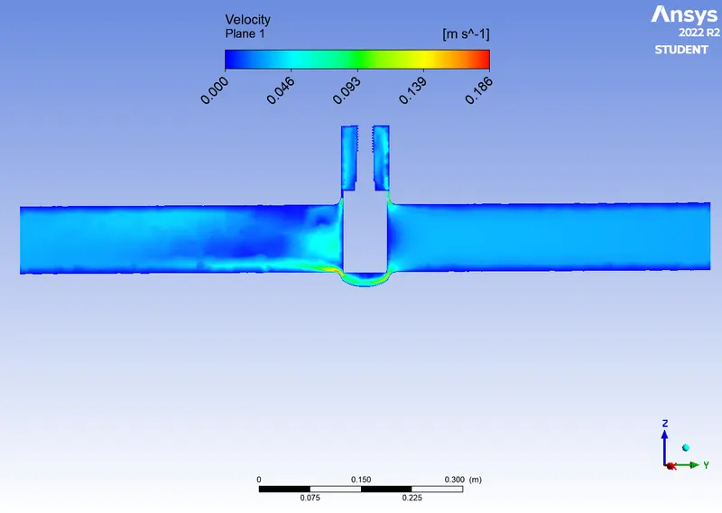
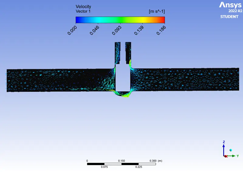
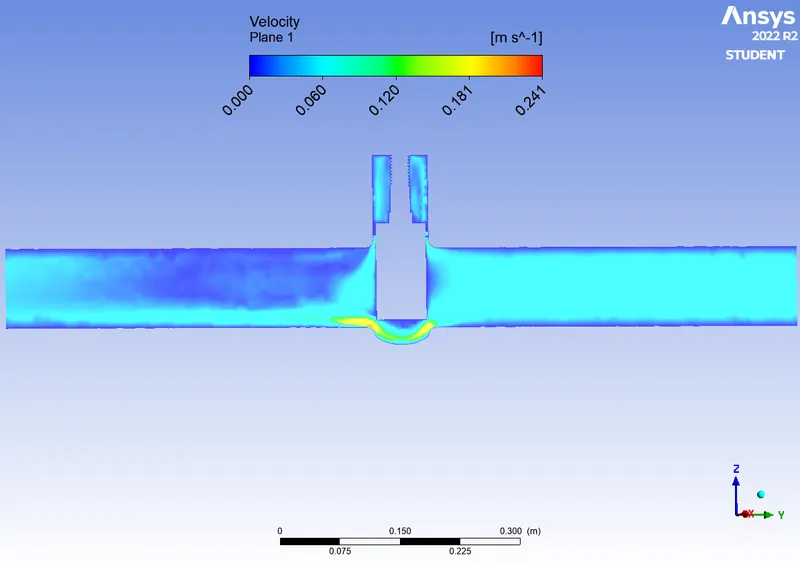
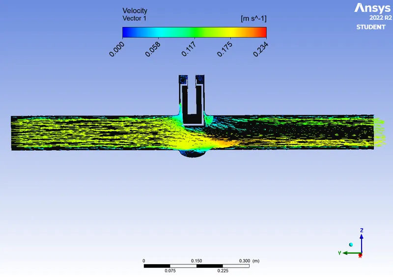
Objective:- Perform the parametric study on gate valve and analyse the mass flow rate and plot the velocity countour.
Thoery:-gate valve, also known as a sluice valve, is a valve that opens by lifting a barrier (gate) out of the path of the fluid. Gate valves require very little space along the pipe axis and hardly restrict the flow of fluid when the gate is fully opened
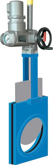
Main parts of Gate valve
1. bonnet
2. spindle
3. gate disk
4. flange
5. handle wheel
CFD:-Computational fluid dynamics or CFD is the analysis of systems involving fluid flow, heat transfer and associated phenomena such as chemical reactions by means of computer-based simulation.
Practical application in current scenario
- aerodynamics of aircraft and vehicles: lift and drag
• hydrodynamics of ships
• power plant: combustion in internal combustion engines and gas
turbines
• turbomachinery: flows inside rotating passages, diffusers etc.
• electrical and electronic engineering: cooling of equipment including
microcircuits
• chemical process engineering: mixing and separation, polymer moulding
• external and internal environment of buildings: wind loading and
heating/ventilation
• marine engineering: loads on off-shore structures
• environmental engineering: distribution of pollutants and effluents
• hydrology and oceanography: flows in rivers, estuaries, oceans
• meteorology: weather prediction
• biomedical engineering: blood flows through arteries and veins
CFD Work Flow:- CFD codes are structured around the numerical algorithms that can tackle fluid flow problems. In order to provide easy access to their solving power all commercial CFD packages include sophisticated user interfaces to input problem parameters and to examine the results
Its threee step process
(i) a pre-processor
involves defination of geometry, grid generation, selection of phenomenon that need to model
(ii) a solver
intergration of governing equation, discretisation and solution
(iii) a post-processor
ploting of contour, graphs and making movies.
In solving fluid flow problems we need to be aware that the underlyingphysics is complex and the results generated by a CFD code are at best asgood as the physics (and chemistry) embedded in it and at worst as good asits operator with CFD
Solving and Modeling Approch:-
There are no way present to understand and analyse the effeciveness of the mixiing tee model.
1. analytical approch
2. simulation approch
3. experimental approch
using analytical approch and experimental approch is time consuming and high cost senario. this could be eliminated by using simulation approch in which we can analyse the system with the actual codition we are intrested in.
To do this we are using ansys fluent solver
we are using fluid flow analysis using Fluent solver because we are interested in the total effectiveness of the fluid in the mechnical tee model, here we are using two different models to analyse the effectiveness of the mixing of fluid.
Approch we are using.
1. We need to open Ansys workbench
2. Choose the Appropiate Solver
3. Assign Appropiate name
4. Choose geometry and select new spaceclaim model.
5. Load the appropiate file
6. Implement the geometrical operation
7. Apply the mesh and provide name selection
8. Choose setup, select the appropiate model
9. Initalisation and running the simulation
10. Result making i.e. countour plots graphs
1. Opening Ansys workbench
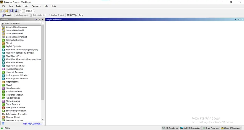
2. Choose the Appropiate Solver
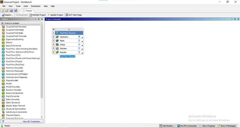
3. Assign Appropiate name:- gate valve
4. Open the file in spaceclaim
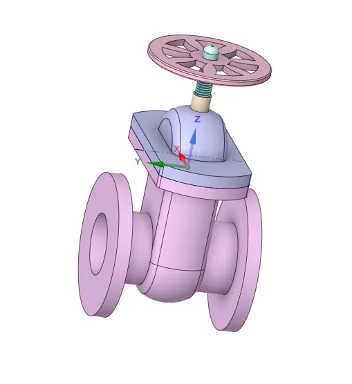
pull the side flanges by 400mm so that we can calculate the mass flow rate
to do this we use pull tool
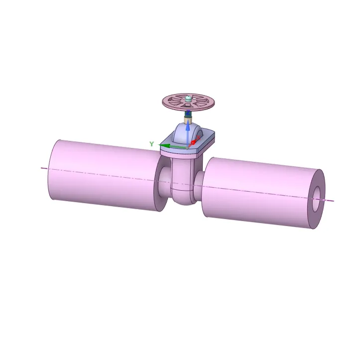
We need to set the parameters
to do this
hide bonnet wheeel and main body
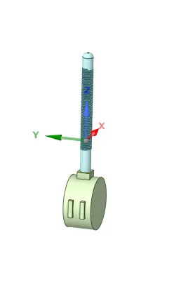
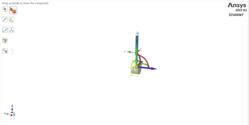
now use move tool to move this by 10 mm
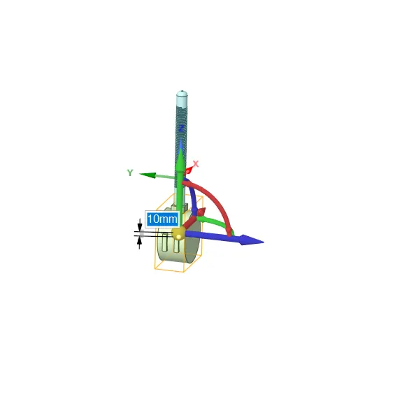
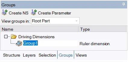
to set this as parameter go to group>create parameter
now extract the volume.
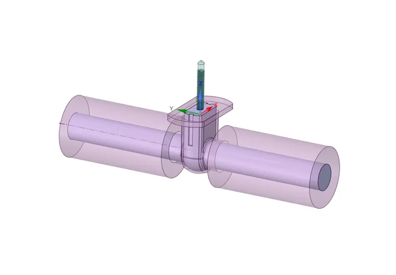
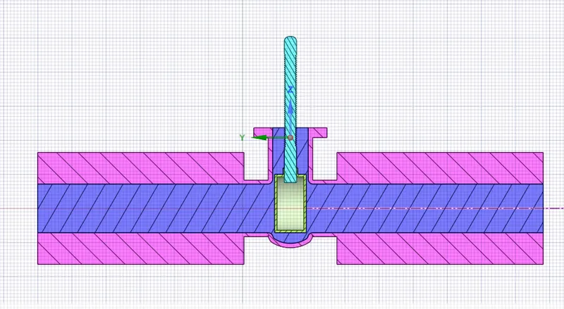
now suppress the solid parts for physics
We done with geometry part
5. Meshing
for meshing we uses the default mesh length
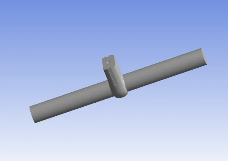
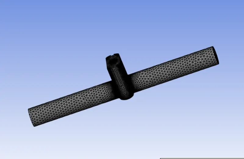
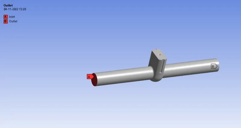
Provide name selection
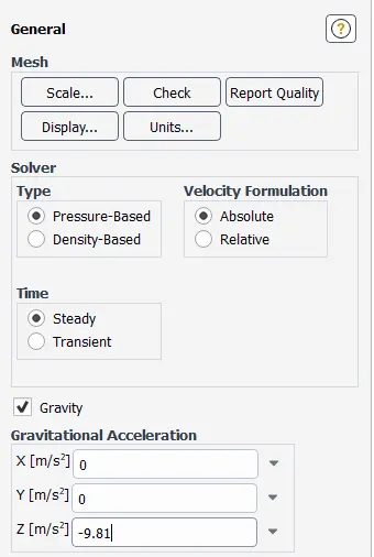
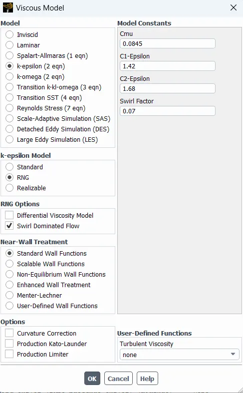
6. Setup
Settings
| Solver | Steady State |
| Energy Equation | Off |
| Model | Laminar,RNZ<SWRIL>Standard |
| Inlet | Pressure Inlet |
| Outlet | Pressure Outlet |
| Material_(Fluid) | Water |
| Cell Zone Condition | Water |
| gravity | Enable in Z direction -9.81m/s^2 |
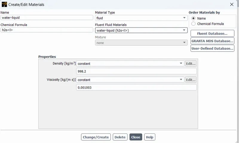
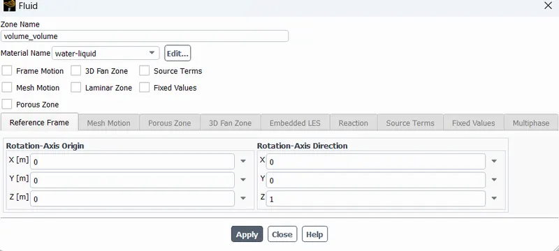
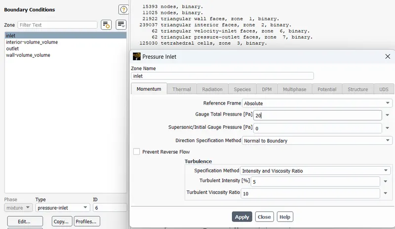
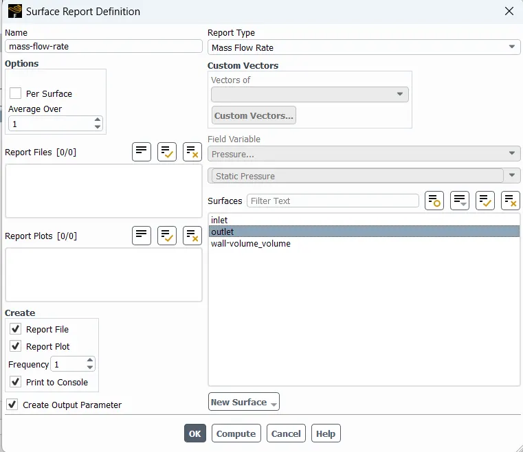
it will create mass flow rate as parametric outlet
Now we can run the simulation for 200 iteration.
7. Parametric Window
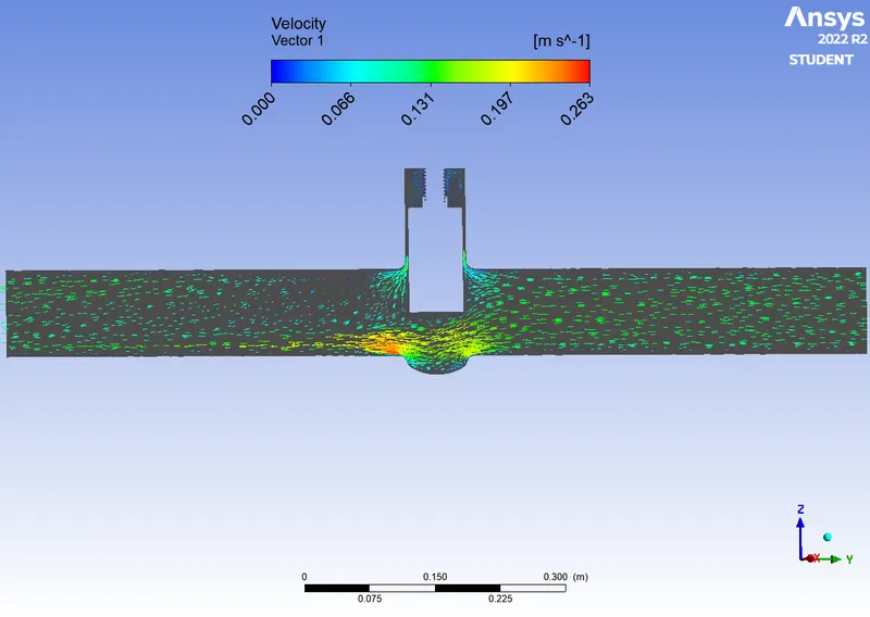
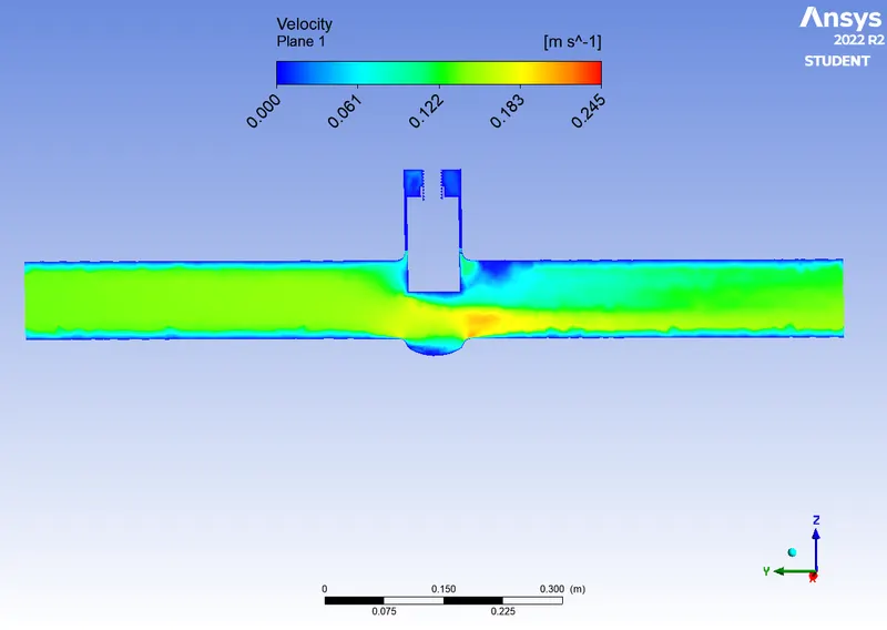
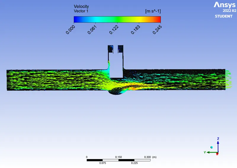
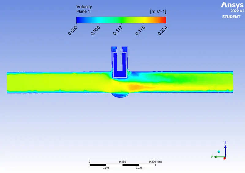
8.Result
For 10mm lift
| Velocity contour | Velcoity Vector |
 |
 |
For 20mm lift
| Velocity contour | Velcoity Vector |
 |
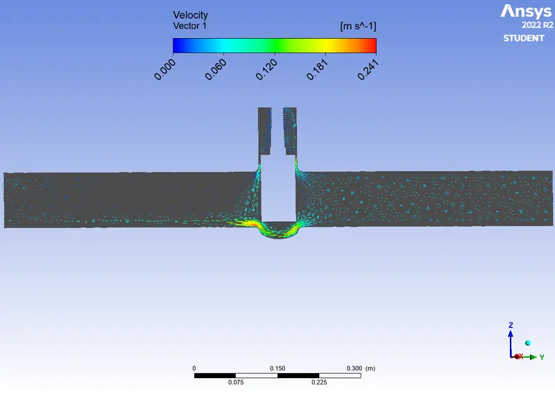 |
For 30mm lift
| Velocity contour | Velcoity Vector |
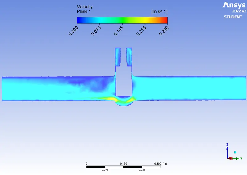 |
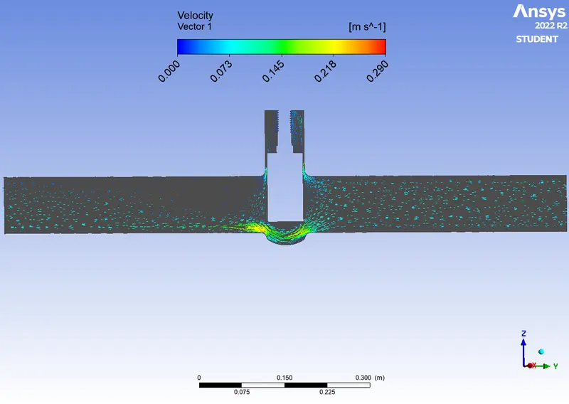 |
For 40mm lift
| Velocity contour | Velcoity Vector |
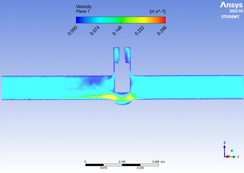 |
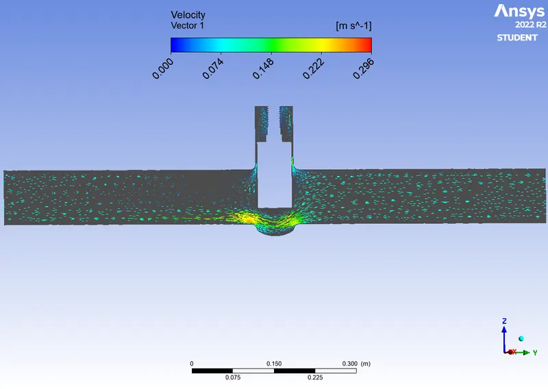 |
For 50mm lift
| Velocity contour | Velcoity Vector |
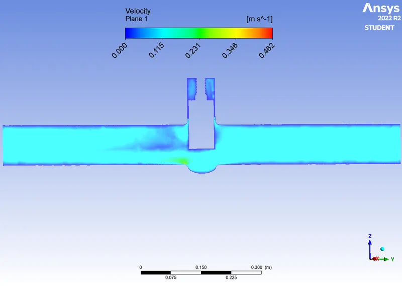 |
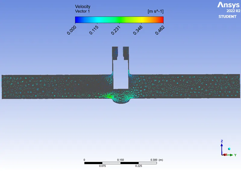 |
For 60mm lift
| Velocity contour | Velcoity Vector |
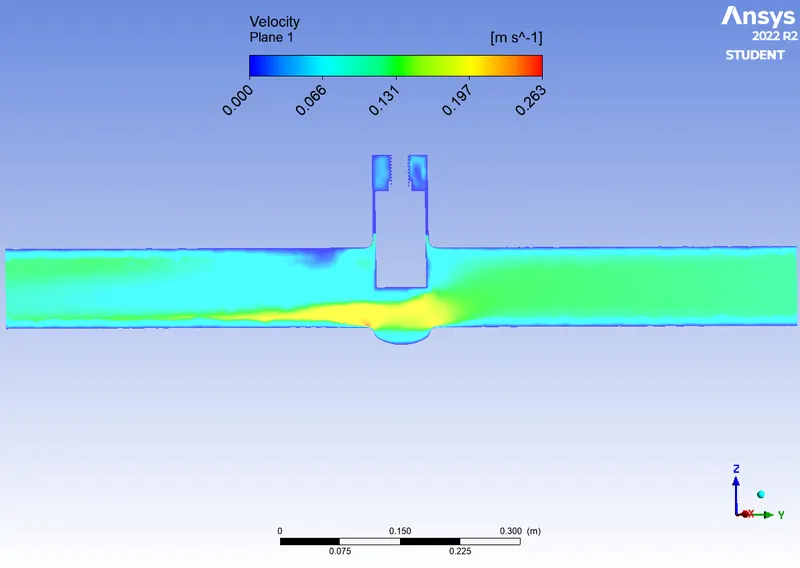 |
 |
For 70mm lift
| Velocity contour | Velcoity Vector |
 |
 |
For 80mm lift
| Velocity contour | Velcoity Vector |
 |
 |
Inferences:-
1. as we increase the valve opening we find that mass flow rate increases
2. as we increase the valve opening we find that velocity decreases
3. as we increases the valve opening overall pressure increases.