Week 4.1 - Genetic Algorithm
AIM:- Code in MATLAB to optimise the stalagmite function and find the global maxima of the function.
Objective:- To find the global maxima of the function.
Theory of genetic algorithum:- GA is a matlab solver, based on random sampling it always tends to minimize the function. In order to find the maxima we need to revert the axis. just by putting minus to the stalagmite function.
CODE:-
%% AIM:- Code in MATLAB to optimise the stalagmite function and find the global maxima of the function.

clear all
close all
clc

x = linspace(0,0.6,150);
y = linspace(0,0.6,150);
num_cases = 50;

%% creating 2dimiensional grid
[xx, yy] = meshgrid(x,y);

%% evaluating the stalagmite function

for i = 1:length(xx)
    for j = 1:length(yy)
        input_vector(1)= xx(i,j);
        input_vector(2)= yy(i,j);
        f(i,j) = stalagmite_func(input_vector);
    end
end


%% study_1 general observation

tic
for i = 1:num_cases
[inputs, fopt_1(i)] = ga(@stalagmite_func,2);
x_opt_1(i) = inputs(1);
y_opt_2(i) = inputs(2);
end

study_time_1 = toc;


%% plotting

figure(1)
subplot(2,1,1)
surfc(xx,yy,-f);
hold on
shading interp; % shading interp is used to hide the grid lines and convert it into  shading
xlabel('X data');
ylabel('Y data');
plot3(x_opt_1,y_opt_2,-fopt_1,'marker','o','markersize',5,'markerfacecolor','y')
legend('surf of f','optimum values(each iteration)')
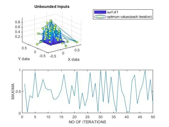
title('Unbounded Inputs')
subplot(2,1,2)
plot(-fopt_1)
xlabel('NO OF ITERATIONS')
ylabel('MAXIMA')


%% study_2 bounding the values

tic
for i = 1:num_cases
[inputs,fopt_2(i)] = ga(@stalagmite_func,2,[],[],[],[],[0;0],[1;1]);
x_opt_2(i) = inputs(1);
y_opt_2(i) = inputs(2);
end
study_time_2 = toc;


%% plotting

figure(2)
subplot(2,1,1)
hold on
surfc(xx,yy,-f)
shading interp
xlabel('X data')
ylabel('Y data')
plot3(x_opt_2,y_opt_2,-fopt_2,'marker','o','markersize',5,'markerfacecolor','r');
legend('surf of f','optimum values(each iteration)')
title('Bounded Inputs')
subplot(2,1,2)
plot(-fopt_2)
xlabel('NO OF ITERATIONS')
ylabel('MAXIMA')


%% study_3 bounding the values and increasing population size

options = optimoptions('ga','populationsize',500);
% options = optimoptions(options,'populationsize',300);
tic
for i = 1:num_cases
[inputs,fopt_3(i)] = ga(@stalagmite_func,2,[],[],[],[],[0;0],[1;1],[],[],options);
x_opt_3(i) = inputs(1);
y_opt_3(i) = inputs(2);
end

study_time_3 = toc;


%% plotting

figure(3)
subplot(2,1,1)
hold on
surfc(xx,yy,-f)
shading interp
xlabel('X data')
ylabel('Y data')
plot3(x_opt_3, y_opt_3,-fopt_3,'marker','o','markersize',5,'markerfacecolor','g');
title('Bounded Inputs with Increased population size');
legend('surf of f','optimum values(each iteration)')
subplot(2,1,2)
plot(-fopt_3)
xlabel('NO OF ITERATIONS');
ylabel('MAXIMA');
FUNCTION CODE:-
function [stalagmite] = stalagmite_func(input_vector)

x = input_vector(1);
y = input_vector(2);

f1_x = (sin(((5.1*pi).*x)+0.5)).^6;
f1_y = (sin(((5.1*pi).*y)+0.5)).^6;

f2_x = exp((((x-0.0667).^2).*(-4*log(2)))./0.64);
f2_y = exp((((y-0.0667).^2).*(-4*log(2)))./0.64);


% f1_x = (sin(5.1*pi).*x +0.5).^6;
% f1_y = (sin(5.1*pi).*y +0.5).^6;
% f2_x = exp((-4*log(2)).*(((x-0.0667).^2)/0.64));
% f2_y = exp((-4*log(2)).*(((y-0.0667).^2)/0.64));

stalagmite = -(f1_x*f1_y*f2_x*f2_y);

endRESULT:-We are getting graphs from LL THE 3 STUDIES.
Study-1
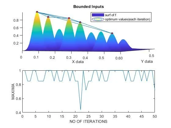
Study-2:- here we introduce the bounds
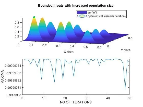
Study-3:- here we increase the populaion size
EXPLANATION:-
GA:- GA is a solver which is used to minimise the given function. GA is always tend to minimise the function. the basic syntax for ga is
Syntax = ga(function, no. of variables,A,b,Aeq,beq,lb,ub,nonlcon,option)
Function:- this is the objective function which is used for actual study or which we have to minimise.
No. of variables:- these are the no. of variables which we have to pass in the ga solver
Linear inequalities:- There are two non-linear equalities.In which we write x variables on the left-hand side of the inequality, and make both inequalities less than or equal. Then we need to convert the equalties in a matrix form.
example
-x(1) -x(2) <= -1
-x(1) + x(2) <= 5
A represent = non linear equalities on left side.
A = [-1,-1; -1,1];
b represent = non linear equalities on right side.
b = [-1;5];
Linear equalities:- There are two non-linear equalities.In which we write x variables on the left-hand side of the inequality, and make both inequalities less than or equal. Then we need to convert the equalties in a matrix form.
example
-x(1) -x(2) == -1
-x(1) + x(2) == 5
Aeq represent = linear equalities on left side.
Aeq= [-1,-1; -1,1];
beq represent = linear equalities on right side.
beq = [-1;5];
Bound:- there are two bounds. Bond is used to define our system on which our study is concentrated. It will a condition which optimise the ga output.
1. upper bonds
upper bond represents by = ub (limits the upper condition)
[1;1]
2. lower bonds
Lower bond represents by = lb (limits the lower condition)
[0;0]
nonlcon:- it represent the inequality and equality. it return value to c and ceq
optimisation option
option= optimoption(function name,'populationsize',300)
output variables:- [inputs, optimum/minimumvalue, exitflag, output]
inputs indicate the coordinate at which ga predict the minimum value.
Program Explantaion:-
1. basic clear all close all and clc this is used to clear all variables close all maps and clc
2. input the varibles as x and y with using linspace
3. with the help of meshgrid command i convert them into 2 dimensional array
4. we create a stalagmite function using given equation
f1_x = (sin(((5.1*pi).*x)+0.5)).^6;
f1_y = (sin(((5.1*pi).*y)+0.5)).^6;
f2_x = exp((((x-0.0667).^2).*(-4*log(2)))./0.64);
f2_y = exp((((y-0.0667).^2).*(-4*log(2)))./0.64);
stalagmite = -(f1_x*f1_y*f2_x*f2_y);
in order to run stalagmite fucntion no f times i uses for loop
5. for i = 1:length(xx)
for j = 1:length(yy)
input_vector(1)= xx(i,j);
input_vector(2)= yy(i,j);
f(i,j) = stalagmite_func(input_vector);
end
end
6. in order to run ga i use for loop again here i uses ending condition as length of numcases
for i = 1:num_cases
[inputs, fopt_1(i)] = ga(@stalagmite_func,2);
x_opt_1(i) = inputs(1);
y_opt_2(i) = inputs(2);
end
fopt_1 = represents the optimum or minimum value for the given function
inputs = represent the x and y values on which ga gives minimum value.
7. i uses tic and toc commad to calculate the operating time/execution time.
8. i created a fingure window and uses subplot commands to plot surf and plot3
figure(1)
subplot(2,1,1) it ll plot graph in 1st row
surfc(xx,yy,-f);
hold on
shading interp; % shading interp is used to hide the grid lines and convert it into shading
xlabel('X data');
ylabel('Y data');
plot3(x_opt_1,y_opt_2,-fopt_1,'marker','o','markersize',5,'markerfacecolor','y') is used to 3 axis graph
legend('surf of f','optimum values(each iteration)')
title('Unbounded Inputs')
9. to plot in 2nd row
subplot(2,1,2)
plot(-fopt_1) it will plot fopt
xlabel('NO OF ITERATIONS')
ylabel('MAXIMA')
10. in similar manner we can execute our 2nd study.
for 2nd study we compile bonds in ga
we just implement the update ga formula with bonds
[inputs,fopt_2(i)] = ga(@stalagmite_func,2,[],[],[],[],[0;0],[1;1]);
Just to limit the fluctuation of the fopt values we are giving the bounds. after setting the upper and lower bonds, we see that the values will fluctuate between the bonds limits.
all unwanted values will terminated.
11. similary we can execute our 3 rd study just by introducing the option
to do that wea are increasing population size increases in order to get better result
option = optimoption('ga','populationsize',500)
and we changed the ga formula.
[inputs,fopt_3(i)] = ga(@stalagmite_func,2,[],[],[],[],[0;0],[1;1],[],[],options);
As we increase the population size we observe that the fluctuation value for fopt will limit to very small interval. as population size increase the fluctuation of fopt reduce and we are getting good result.
ERROR:- The only error i get is beacuse
i use this
stalagmite = (f1_x*f1_y*f2_x*f2_y);
After using the above mentioned formula m getting plot in Negative z-direction which is not correct. it represent the minima
surf we are getting for study_1 is very little or less visible
for plot of Maxima vs no of iteration we are getting straight line or constant value for each iteration which is not correct.
instead of this
stalagmite = -(f1_x*f1_y*f2_x*f2_y);
After using the above mentioned formula m getting plot in positive z-direction which is correct. it represent the maxima
for plot of Maxima vs no of iteration we are getting fluctuating values for each iteration which is correct.
to overcome this i took one on one session.