Week 9 - Parametric study on Gate valve.

Abstract

The following project is a simulation report of flow of water through a gate valve with different opennings. The mass flow rates for the different valve openings is calculated. The pressure drops are calculated. A parametric study is underwent for gate valve opening from 10% to 80%.

Key words : gate valve, parametric study, ANSYS FLUENT, mass flow rate

Introduction

A gate valve, also known as a sluice valve, is a valve that opens by lifting a barrier (gate) out of the path of the fluid. Gate valves require very little space along the pipe axis and hardly restrict the flow of fluid when the gate is fully opened.

A gate valve is generally used to completely shut off fluid flow or, in the fully open position, provide full flow in a pipeline. Thus it is used either in the fully closed or fully open positions.

CFD analysis flow chart

1) Geometry preparation

2) Meshing

3) Fluent set up and solving , parametric study

4) Post-processing

1) Geometry preparation:

A stepfile is loaded into ansys space claim. Here only the fluid flow is simulated, so the fluid volume needs to be extracted only. The unnencessary parts me be deleted that do not take part in the simulation set up. The bonnet, the hand wheel is deleted. The bottom solid part is pulled outwards using the pull option in the desighn window. The prepare window enables us with volume extraction option.With the help of edge selection tool and using the edge selection method, the fluid volume i extracted .

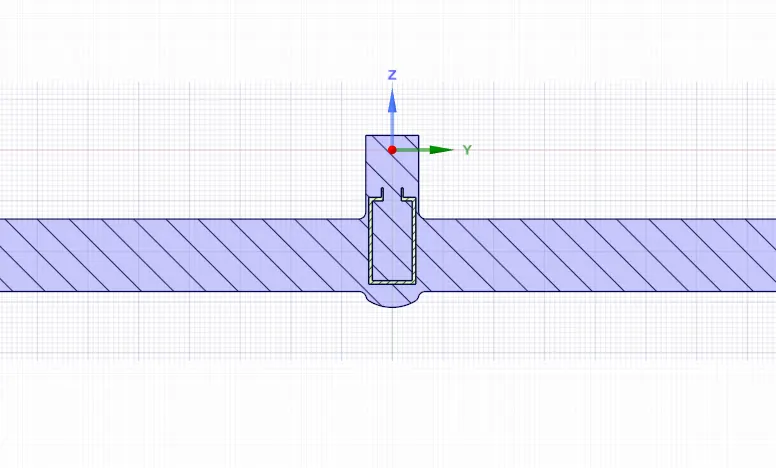
Here to regukate the openning of the gate valve, the gate disk needs to be parametricized. It is moved by a 0.01 meters in the y direction using the move tool in the design window. parameter is added.

The geometry is now ready to be transferred for the meshing module.

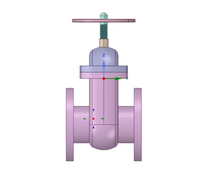
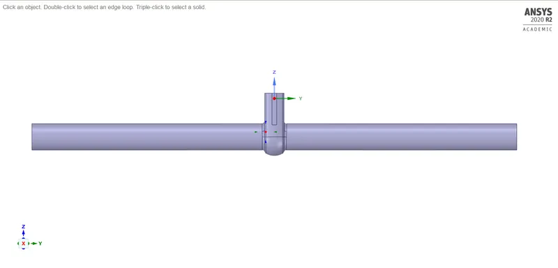
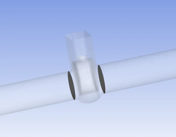
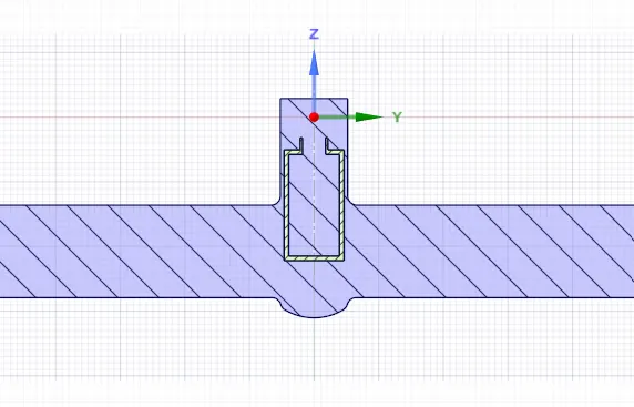
The first image is of the complete gate valve , the second one is of the extracted volume that will be analysed for fluid flow.

2) Meshing:

A general mesh is applied , with sizing of 0.01 meters. Since academic version of Ansys is used, there is a upper limit to the number of elements that can be reached.

element size	0.01
nodes	38583
elements	192164

Element quality:

minimum	0.22763
maximum	0.99988
average	0.83614
standard deviation	9.5001e-002

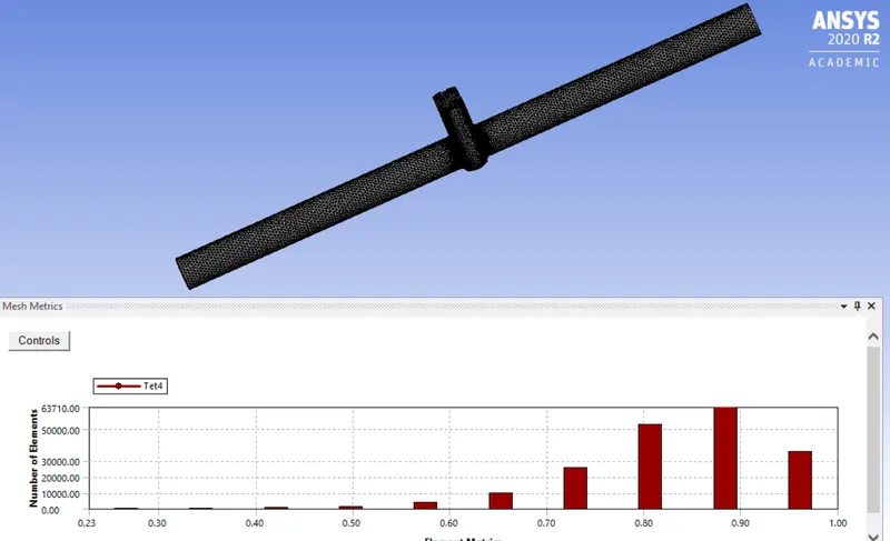
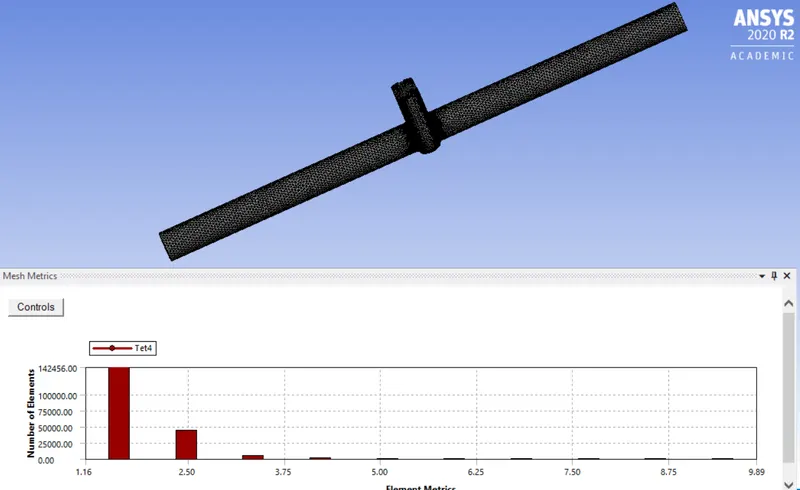
Aspect ratio:

minimum	1.1597
maximum	9.808
average	1.8536
standard deviation	0.45816

Skewness:

minimum	3.92e-005
maximum	0.78691
average	0.22972
standard deviation	0.11987

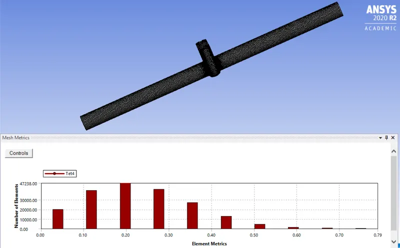
Orthogonal quality:

minimum	0.21039
maximum	0.99124
average	0.76883
standard deviation	0.11759

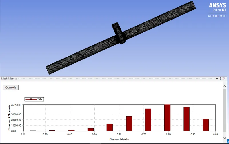
3) Fluent set-up:

After the geometry is meshed and proper named selection os done to the inlet and the outlet; Fluent is openned to set up the physics and the the flow.

Steady state analysis is selected.

Pressure based solver is opted for

The orientation of the geometry is such that, the accelaration due to gravity is turned on and along the Z axis, -9.81 m/s^2 is the value put in.

Turbulence modelling:

The model selected is realizable K-epsilon with scalable wall functions.

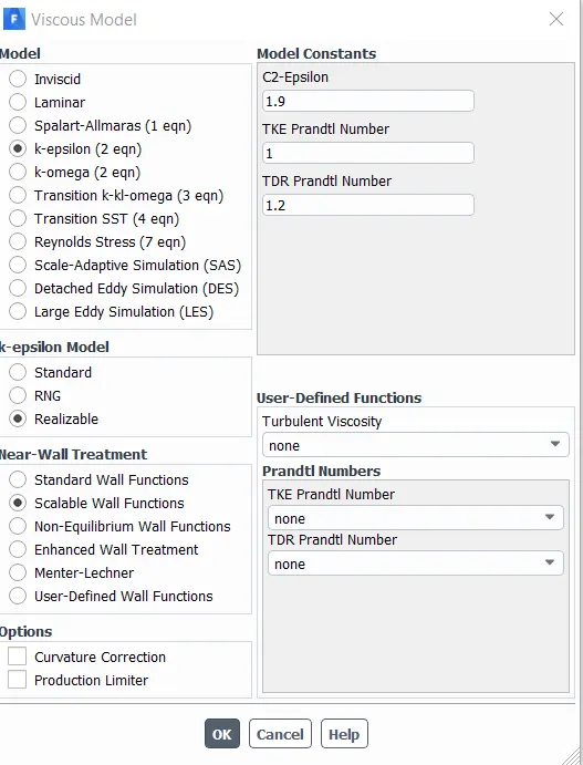
Here the working fluid is water. From the fluent database, water is selected (liquid). Opening the cell register, the working fkuid in the fkuid volume is changed to water (liquid) . By default Fluent assumes air as the working fluid.

Boundary conditions:

Here the inlet is pressure inlet. Total gauge pressure at the inlet is 10 pascals .

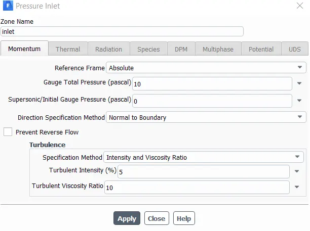
The outlet is a pressure outlet.

The velocity at the inlet is calculated during Standard initializaton from the inlet. The velocity came out to be 0.1415 m/s. Output parameter is created for the mass flow rate. Here since a parametric study is done for various valve openings.

Number of iterations =500

Solution methods:

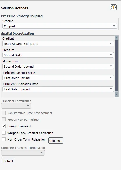
A coupled pressure velocity coupling scheme is selected.

4) Results :

Calculation of Reynolds number :

`Re = ((rho)*(V)*(D))/(mu)`

Here , `rho`is the density of the fluid (water)

`V`is the velocity of the fuid at the inlet

`D`is the diameter f the pipe

`mu` is the viscosity of water

Density of water	998 kg/m^3
Inlet velocity	0.1415 m/s
Diameter of the pipe	0.1 meters
Dynamic viscosity of water	1.793*10^-3 kg/(ms)

So, Reynolds number = 7876

For Reynolds number > 4000, the flow is turbulent in pipe flows. So this is a case of turbulent flow.

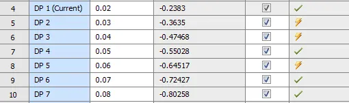
The parametric study was performed for various valve openings from 0.01 meters to 0.08 meters . The corresponding mass flow rates at the outlet was obtained .

Flow coefficient: This is a measure of a valves efficienc at allowing fluid flow through the arrangement. This is a relationship between the pressure drop across an valve and the corresponding flow rate .

`Cv= (Q)*((SG)/(dP))^(1/2)`

Here,

`Cv`is the flow coefficient ,

`Q`is the rate of flow in US gallons/minute

`SG`is the specific gravity of the fluid that flows through the valve ( in this project, it is water)

`dP`is the pressure drop ,in psi

Cv is the volume of water at 60 degree farenheit that will flow per minute through a valve with pressure drop of 1 psi cross the valve.

To convert , pa into psi , and kg/s to US gallons /minute

1 pa = 0.00014503 psi

1 kg/s = 21.44 (gal/min).

In SI system, Flow factor `Kv`is intoduced.

`Kv=(Q)*((SG)/(dP))^(1/2)`

here ,

`Q`is in m^3/h

`Kv`is volume of water flow in m^3/h at a pressure drop across the valve of 1kgf/cm^2when the valve is completely open.

Emperically, `Kv=0.865*Cv`

To find out the pressure drop, Ansys post is openned ,

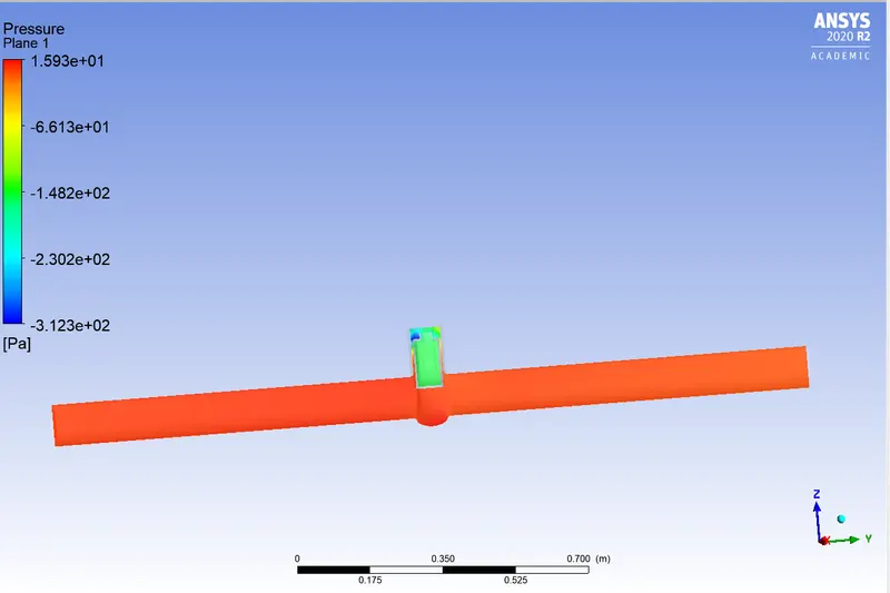
To find out the pressure drop. Two planes are created in the vicinity of the gate valve by using the create plane option. On these two planes , the average pressure are calculated from the function calculator option.

Plane definition :

plane 2: location ZX plane and at a distance of 0.053 meters

plane 3 : location ZX plane and at a distance of -0.053 meters

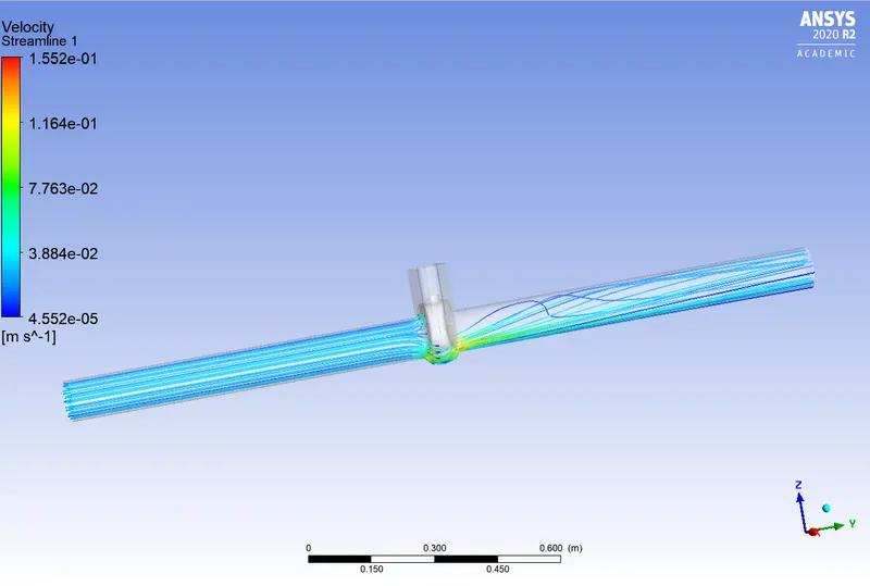
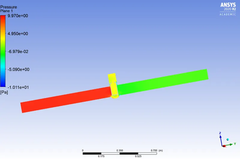
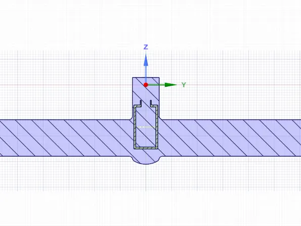
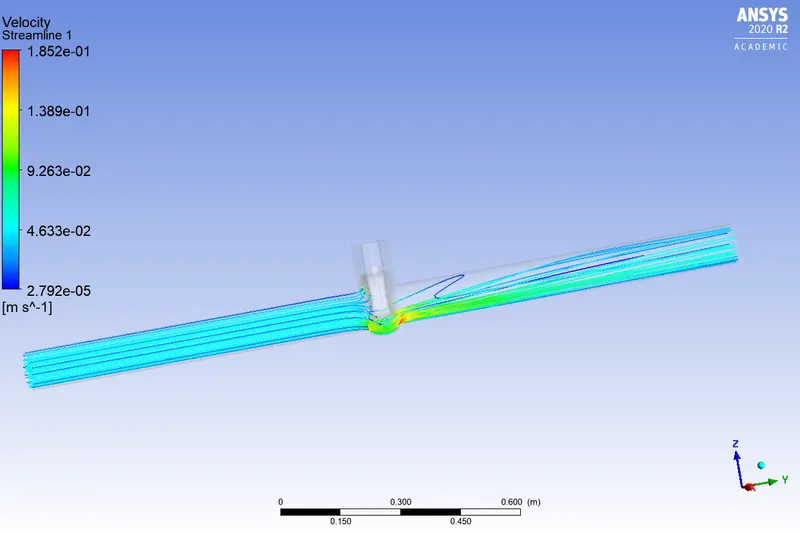
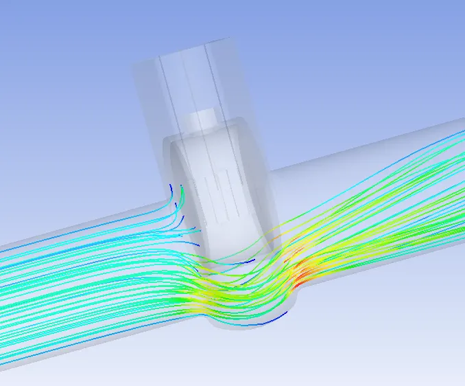
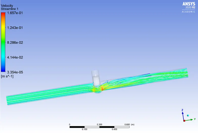
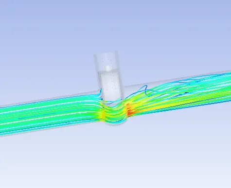
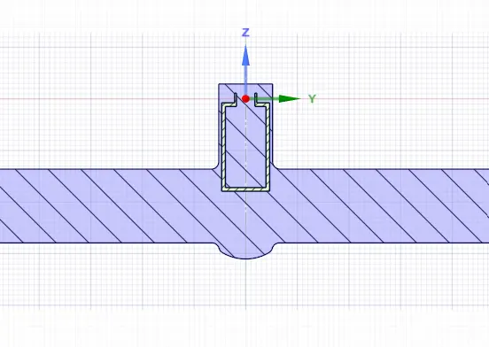
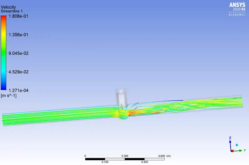
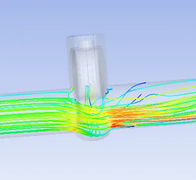
Each valve opening is tabulated below with the sectional view and the corresponding pressure drops and mass flow rates.

valve opening(meters)	pressure drop(pa)	mass flow rate(kg/s)	Q (in US gallons/minute)	pressure drop in psi	Cv(gal/min)	Kv(m^3/h)
0.01	10.1987	0.1487	3.188	1.479*10^-3	82.896	71.70
0.02	10.3000	0.2383	5.109	1.493*10^-3	132.225	114.37
0.03	10.2852	0.3635	7.793	1.491*10^-3	201.820	174.5743
0.04	9.49778	0.4746	10.175	1.377*10^-3	274.199	237.182
0.05	7.39742	0.5520	11.834	1.072*10^-3	361.438	312.643
0.06	6.62986	0.6451	13.830	9.6151*10^-4	446.010	385.798
0.07	4.71609	0.7242	15.526	6.8396*10^-4	593.668	513.522
0.08	4.56617	0.8025	17.205	6.6223*10^-4	668.575	578.317

Valve opening 0.02 meters:

Valve opening 0.03 meters:

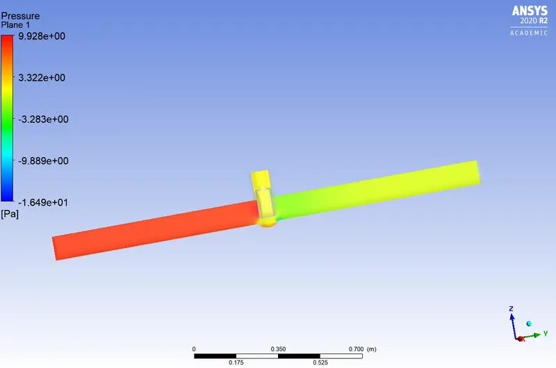
Valve opening 0.04 meters:

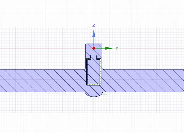
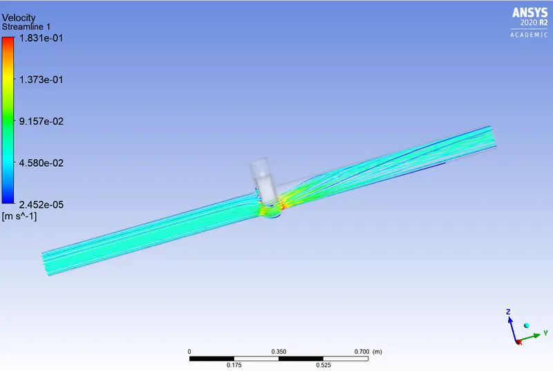
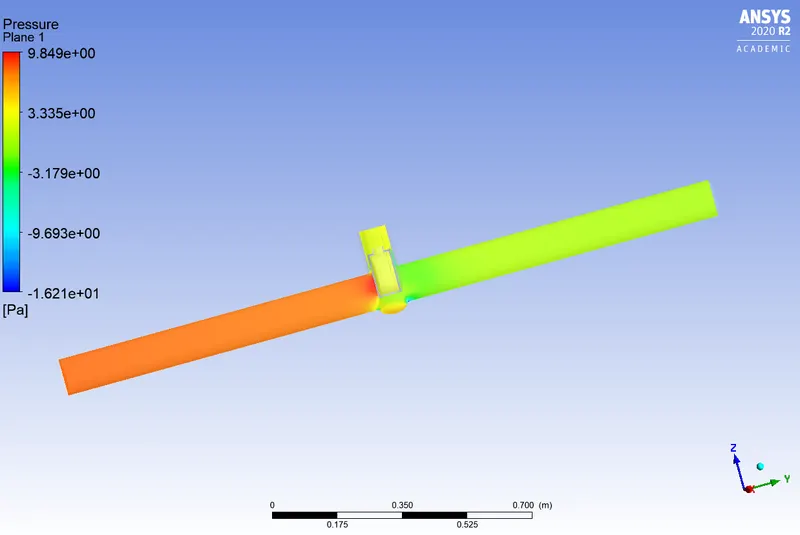
Valve opening 0.05 meters:

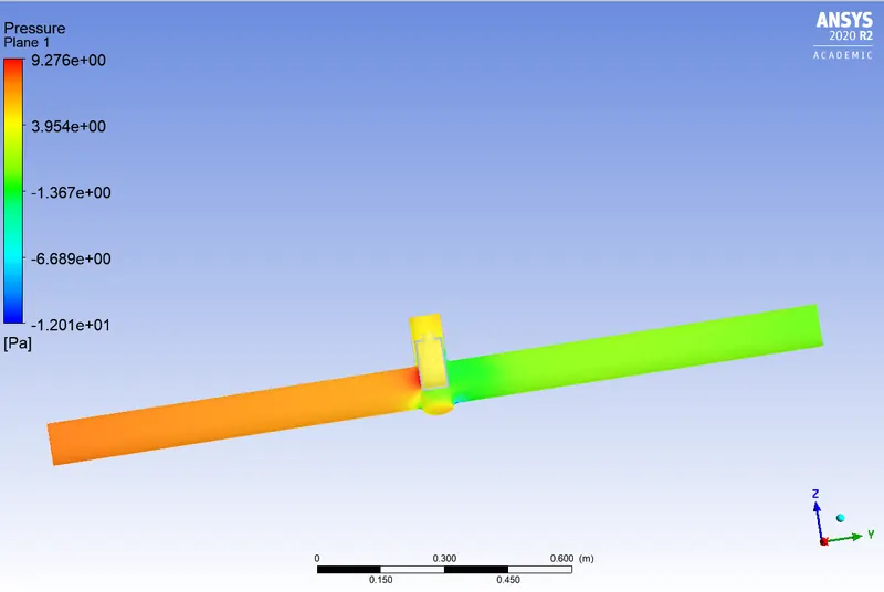
Valve opening 0.06 meters:

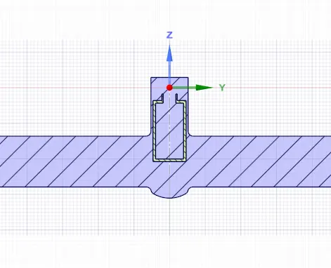
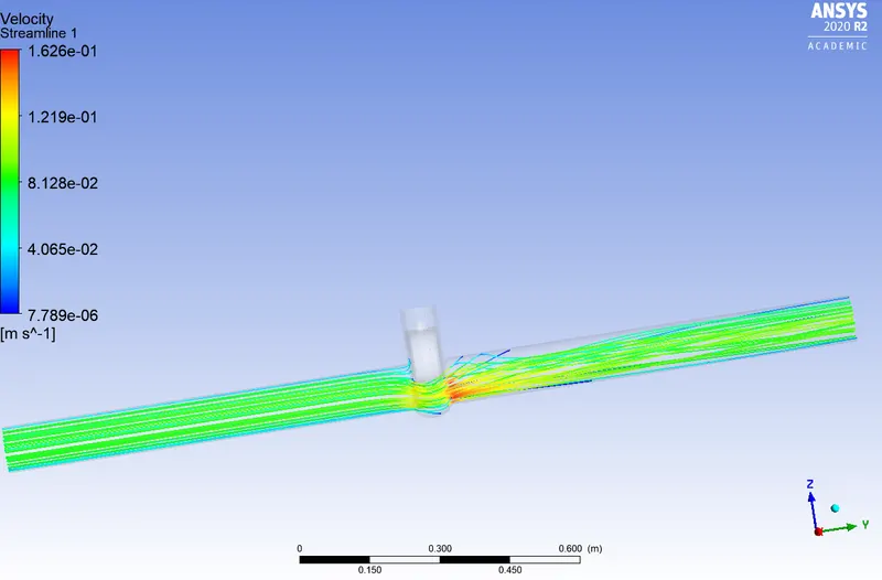
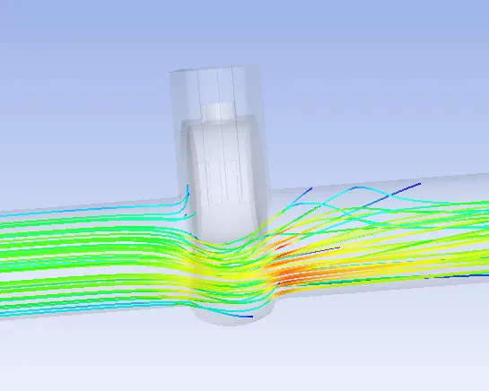
Valve opening 0.07 meters:

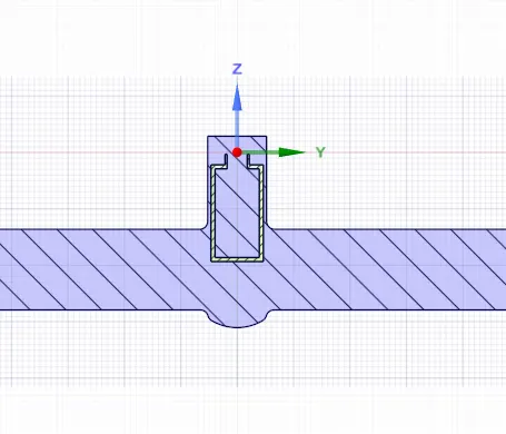
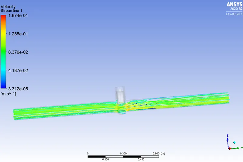
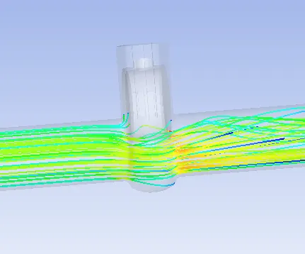
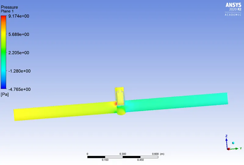
Valve opening 0.08 meters:

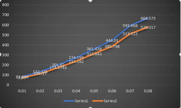
plot of Flow coefficient and flow factor withrespect to valve openings:

The valve openings are plotted along the X-axis. From 0.01 meters to 0.08 meters . Along the Y axis are the Cvand Kv. The blue line represents the Flow coefficient (Cv) The orange line represents the Fow factor (Kv).

The line plot is prepared in microsoft excel.

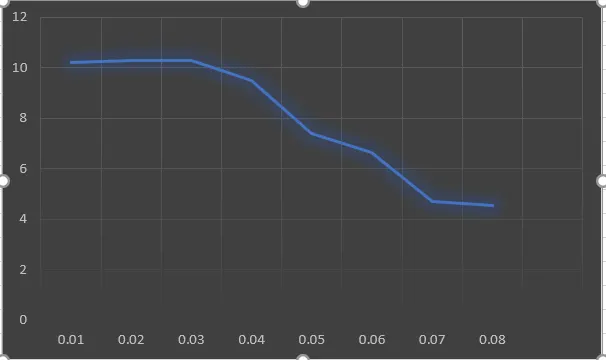
The second plot is between pressured drop vs the valve openings. Pressure drop is plotted on the Y axis

Conclusion:

• With the increase in valve openings, the pressure drop reduces
• With the increase in the valve openings , the mass flow rate at the outlet increases too.
• The increase in velocity just in the vicinity of gate valve can be attributed to the equation AV = constant. With the decrease in the flow area due the valve to maintain the same flow rate, the velocity increases.
• Both the flow coefficient and the flow factor increases with the increase in the valve opening from 0.01 meters to 0.08 meters.