Parametric analysis of flow through a gate valve.
I. Aim: To perform a parametric analysis of flow through a gate valve and to analyze the effect of gate valve opening on the mass flow rate.
II. Introduction:
In any numerical simulation, it would be time-consuming for repeating the same analysis for variation in input parameters like geometry dimension changes, changes in boundary condition values, etc. The parametrization of these quantities in ANSYS Workbench helps us to simulate various scenarios of input changes without actually repeating all the usual setup steps. The effect of variation of any input quantities on output quantities can be analyzed by parametrization of the interested input and output quantities in ANSYS Workbench.
For example, if we want to analyze the effect of different wind velocities on the drag force acting on a vehicle, the input velocity parameter and output drag force parameter can be parametrized. It would be sufficient to set up and run any-one initial design point, then the solution can be updated to any number of design points just by specifying the respective input parameter in the ANSYS Workbench parameters tab and updating the solution.
In this project, a parametric analysis of flow through a pipe gate valve is simulated using ANSYS Workbench. The parameters of interest are the gate valve lift and outlet mass flow rate. The effect of gate valve opening to different heights on the outlet mass flow rate of water is analyzed using Parametric analysis.
III Objectives:
perform a parametric study on the gate valve simulation by varying the opening from 10 mm to 80 mm from its initial position.
- Obtain the mass flow rates at the outlet for each design point.
- Calculate the flow coefficient and flow factor for each opening and plot the graph.
- Discuss the results of the mass flow rate and flow coefficient.
IV: Solving & Modelling approach:
3D steady-state CFD analysis is carried out in Ansys workbench using a Fluent solver to simulate the flow through the gate valve. Water is used as the fluid flowing through the gate valve. Initially, the gate valve is opened for a 10 mm lift from its initial position and the outlet mas flow rate is determined. Then these inlet and outlet quantities are parametrized for other design points.
V: Pre-processing and solver setting:
The first step in a CFD analysis is preprocessing. This includes preparing the geometry/ computational domain, discretization of the domain (meshing), assigning material properties, boundary conditions, creating input and output parameters of interest, and solver setup.
1. Geometry/Domain:
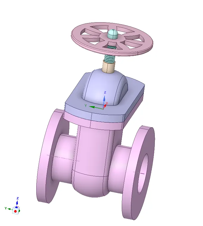
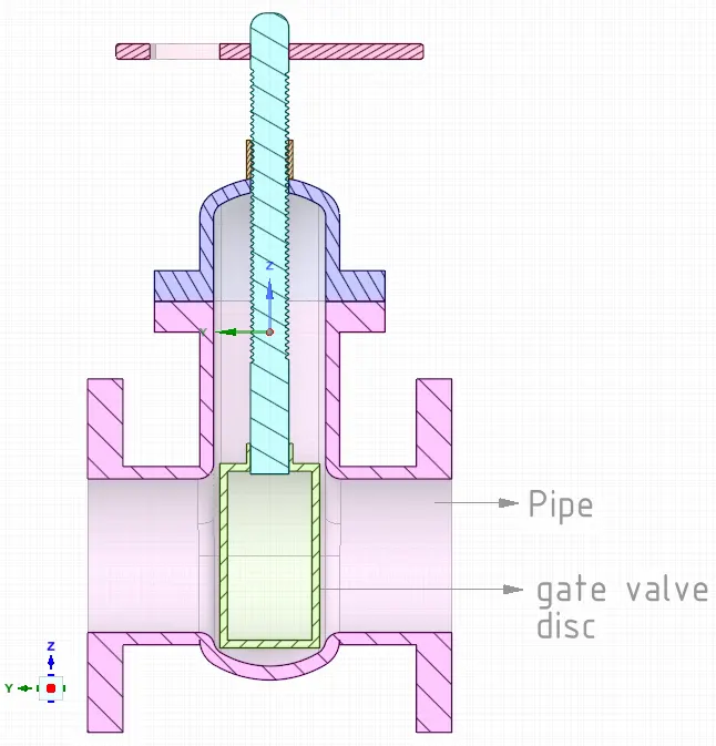
A 3D solid geometry of the typical gate valve of a pipe is imported into Spaceclaim. It consists of components like a disc, spindle, valve opening wheel, etc. The geometry is shown below:
| 3D-Gate valve geometry | Section view |
 |
 |
The gate valve disc is moved from its initial position to the 10 mm (first design point ). Also, a parameter is created for this disc opening dimension (by creating a parameter in the group tab in SpaceClaim) as shown in the below figure.
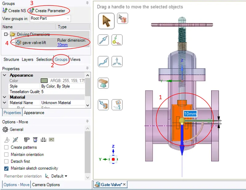
This would create the input parameter of valve opening height. A parameter set is created instantly on the Workbench project page. Various design points can be added in the parameters tab.
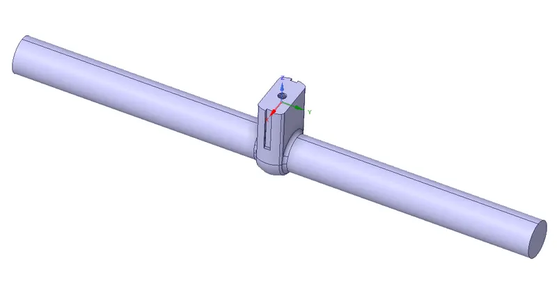
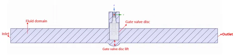
After the parameter is set for the gate disc opening, the pipe section of the valve is extended and a fluid volume is extracted using the volume extraction option. The extracted volume details are shown in the below figures.
| Extracted fluid volume | Section view |
 |
 |
2. Domain discretization /Meshing:
The 3d fluid domain is discretized into a finite number of control volumes using the Ansys meshing component. The following table shows the mesh details:
| Property | Value |
| Global element size | 30 mm |
| Cell count | 122586 |
| Element quality | 0.82 |
The cell zones and boundaries of the domain are also defined in the Ansys mesher using the named selection option. The boundaries are defined as follows:
| Boundary/Cell Zone | Boundary/Cell Zone name |
| Inlet | inlet |
| Outlet | outlet |
3. Solver setup:
The 3D analysis is performed on the discretized domain(meshed model) in Ansys Fluent CFD software. A double-precision parallel solver with 4 cores is used. The double-precision solver uses 64-bit precision, which reduces the round-off error in the results. The solver setup details are given below:
| Solver type | Steady-state pressure-based solver |
| Gravity effect | '-ve' Y-direction, 9.81 m/sec^2 |
| Turbulence model | realizable `k-epsilon` with scalable wall function |
| Fluid domain | Air (default Ansys fluent properties) |
| Pressure - Velocity Coupling | Coupled |
| Residual Monitors Criteria | 1E-03 for all the governing equations |
Boundary Condition:
| BC | |
| Inlet | Pressure inlet (gauze pressure - 10 Pa) |
| Outlet | Pressure outlet (gauze pressure - 0 Pa) |
VI Solution:
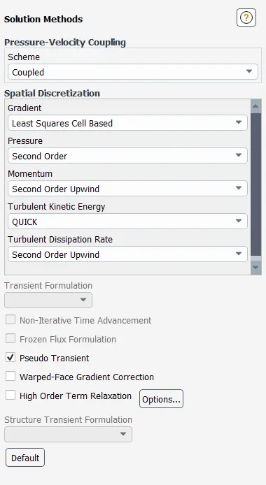
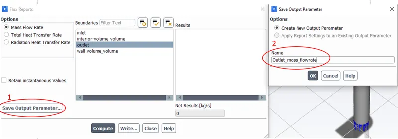
The solution is initialized with standard initialization with computing from the inlet. The solution is run for 700 iterations. The outlet mass flow rate which is the parameter of interest, is parametrized as shown below:
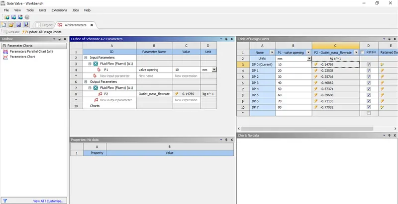
The first design point is solved and then the solution is updated to other design points in the parameters tab as shown in below image:
VII Results:
The parametric analyses of flow through a gate valve in a pipe section is carried in this analysis. The parameters of interest are gate valve disc opening and outlet mass flow rate of water. Initially, the analysis is run for 10 mm lift of gate valve opening and the mas flow rate is found out. Then using the parametric option available in ANsys Workbench, more design points are added with increasing gate valve opening height and the corresponding outlet mass flow rate is found as shown in below table:
| Valve Opening (Z direction lift) (mm) |
Outlet Mass flow rate (kg/sec) | volume flow rate (m^3/sec) | volume flow rate (U.S gal/min) | Inlet Pressure (Pa) | Outlet Pressure (Pa) | Pressure drop (Pa) | Pressure drop (Psi) | Flow Coefficient -Cv (U.S gal/min) | Flow factor -Kv (m^3/hr) |
| 10 | 0.1476 | 1.48E-04 | 2.193 | 9.81766 | 0 | 9.81766 | 1.42E-03 | 58.1238877 | 50.27716286 |
| 20 | 0.2353 | 2.35E-04 | 3.495 | 9.53666 | 0 | 9.53666 | 1.38E-03 | 93.98612453 | 81.29799772 |
| 30 | 0.3571 | 3.57E-04 | 5.304 | 8.93358 | 0 | 8.93358 | 1.30E-03 | 147.3466907 | 127.4548875 |
| 40 | 0.4686 | 4.69E-04 | 6.959 | 8.16554 | 0 | 8.16554 | 1.18E-03 | 202.2175673 | 174.9181957 |
| 50 | 0.5737 | 5.74E-04 | 8.520 | 7.22859 | 0 | 7.22859 | 1.05E-03 | 263.1259594 | 227.6039549 |
| 60 | 0.5968 | 5.97E-04 | 8.864 | 7.14797 | 0 | 7.14797 | 1.04E-03 | 275.2894007 | 238.1253316 |
| 70 | 0.7110 | 7.11E-04 | 10.559 | 5.77512 | 0 | 5.77512 | 8.38E-04 | 364.8486459 | 315.5940787 |
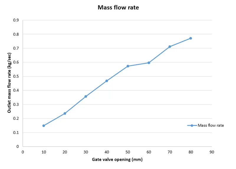
It can be seen that, the mass flow rate increases from 0.147 kg/sec to 0.711 kg/sec, when the gate valve opening is increased from 10 mm to 80 mm height from its initial position. Also, the above table gives the flow coefficient (Cv) and flow factor (Kv), which are explained as below:
Flow Coefficient:
The flow coefficient (Cv) of a device is a relative measure of its efficiency at allowing fluid flow. It describes the relationship between the pressure drop across an orifice/opening of valve or other assembly and the corresponding flowrate.
Mathematically the flow coefficient Cv (or flow-capacity rating of valve) can be expressed as :
`C_v = Q*(sqrt((S.G)/(DeltaP)))`
where:
- Q is the rate of flow (expressed in US gallons per minute),
- S.G is the specific gravity of the fluid (for water = 1),
- ΔP is the pressure drop across the valve (expressed in psi)
The use of the flow coefficient offers a standard method of comparing valve capacities and sizing valves for specific applications that is widely accepted by industry.
Flow factor:
The metric equivalent of flow coefficient is the flow factor (Kv) is calculated using metric units and is given by the relation:
`K_v = Q*(sqrt((S.G)/(DeltaP)))`
where
- Kv is the flow factor (expressed in m^3/hr).
- Q is the flow rate (expressed in cubic metres per hour m^3/hr]),
- S.G is the specific gravity of the fluid (for water = 1),
- ∆P is the differential pressure across the device (expressed in [bar]).
Kv can be calculated from Cv using the equation:
- `K_v = 0.865*C_v`
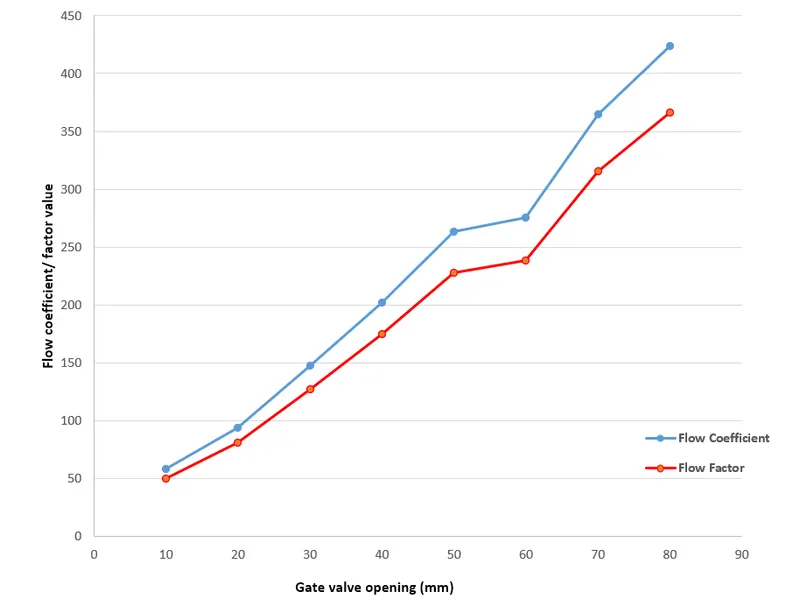
The flow coefficient and flow factor increases as the gate valve opening is increased, as the volume flow rate through the valve increases as shown in the above table.
The effect of valve opening on the outlet mass flow rate, flow coefficient and flow factor is represented graphically in the below plots:
Conclusion:
The main objective of this project is to perform a parametric analysis in ANSYS Workbench. The flow through a pipe gate valve is analysed by parametrizing the gate valve opening and its effect on the outlet mass flow rate, flow coefficient and flow factor. The parametric analysis option helps in greatly reducing the pre-processing and post-processing computational time when performing the same analysis for different design points. In the current analysis of water flow through agate valve, outlet mass flow rate, flow coefficient and flow factor increased as the valve opening is increased due to greater volume flow through the valve.
References:
2. https://skill-lync.com/knowledgebase/parametrizing-in-ansys-fluent
3. https://skill-lync.com/knowledgebase/gate-valve-parametric-study-help