Week 9 - Mini project - Flow over an Airfoil

Objective:

To set up a simu;ation over a NACA 2412 aerofoil and to find out the following

• Drag co-efficient Vs Angle of Attack
• Lift co-efficient vs Angle of Attack
• Compare the effect of turbulence models on the above two results.
• Make sure that the inlet Reynolds number is 200,000
• calculations for the following angle of attacks,
  • Angle of attack = 1º
  • Angle of attack = 5º
  • Angle of attack = 10º
  • Angle of attack = 15º

Theory :

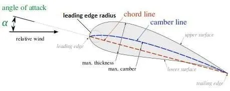
The above image shows the standard nomenclature of an airofoil.

Aerofoil is the cross section of the wing normal to the span .The span of the wing is the lateral length of the aircraft. the distance between the two tips of the aircraft is called the span.

The camber of the upper surface is more pronounced than the camber of the lower surface which is lot flatter.

Angle of attack: It is the angle between the relative wind and the chord line.

chord is the distance between the leading edge to trailing edge

Aspect ratio: The ratio between the wing span and the mean chord is called the aspect ratio .

An aerofoil is a streamlined body designed in such a way that the separation occurs at the extreme rear end of the body. Such that it produces small wake and subsequently small pressure drag. Even for high reynolds number the pressure drag is very small, the skin friction drag makes major contribution to the drag component as a whole.

In case of aerofoils, the resultant force is perpendicular to the direction of the flow. It is called as lift.

In case of NACA 2412 , the first two digits, signifies the camber of the aerofoil and the last two digits signifies the thickness.

The aerofoil is 12% thick and maximum camber is 0.02c at x=0.04c , c denotes the chord length.

If we apply Bernoulis principle at two sections of the aerofoil, The upper part and the lower part.

`(P_u)/(rho)+(0.5*V_u^2)=(P_l)/(rho)+(0.5*V_l^2)`

here , `P_u, V_u` denotes the pressure and velocity at the upper section and `P_l,V_l` denotes the pressure and velocity at the lower part. The velocity at the upper part is more than the velocity of the lower part. So, the pressure at the upper part is less than the pressure at the lower part. This pressure difference created generates the lift in the aerofoil.

The lift coefficient , `C_l=(F_l)/(0.5*rho*V^2*A_p)`

here , `F_l`is the lift force , `A_p` is the area of the frontal projection.

Similarly the drag coefficient is given by: `C_d=(F_d)/(0.5*rho*V^2*A_p)`

Here `F_d`is the drag force .

Geometry set up:

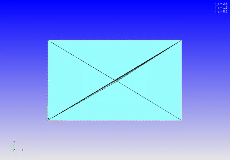
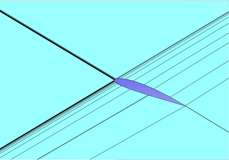
The aerofoil is generated from the co ordinates of the areofoil , After the co ordinates are plotted, they are patched. To create the 2D surface, the surface created from the co ordinates are copied and given an offset of 1 meter in the z direction.

To set up aerodynamic simulations , it is important to create wind tunnels. The length of the wind tunnel is conventionally taken as the fifty times the chord length. The breadth or height of the wind tunnel is conventionally taken as thirty times the chord length.

The idea is to , create an exact shape of the aerofoil inside the wind tunnel and carry out the simulation.

Case set up:

• Application type : Time based
• Materials :

Preffered mixture is Air. Gas simulation is checked and the species box is checked. The species are selected as O2 and N2.

Global transport parameter:

Turbulent Prandtl number	0.9
Turbulent schmidt number	0.78

• Simulation parameters:

Run parameters:

Transient simulation is done , with a full hydrodynamic case and the gas flow solver is compressible.

Simulation time parameters:

Calculation of end time :

Flow through time = (Length of tunnel/Velocity of flow)

Velocity of flow is calculated from the Reynolds number:

`Re=(rho*V*D)/(mu)`

here, `rho,D,mu,Re`is known, from that , the velocity of flow is calculated.

V is calculated to be 30.14 m/s

Now the length of the tunnel created is 2.5 meters.

So the flow through time is (2.5/30.14) =0.08 seconds. generally the simulation end time is calculated as four to five time sthe flow through time. So the simulation end time is 0.5 seconds

Initial and minimum time steps are 1e-05 seconds. maximum time step is 1 seconds.

Maximum convection CFL limit is 1 . maximum diffusion CFL limit is 2.

Solver parameters:

Navier stokes solver scheme is seklected as PISO and density based solver is used.

• Boundary conditions:

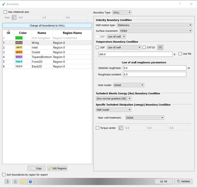
1) Wing :

Boundary type : Wall

velocity boundary condition:

Wall motion type : stationary

Surface movement : fixed

Law of wall prevails.

Temperature boundary conditions: Law of wall prevails.

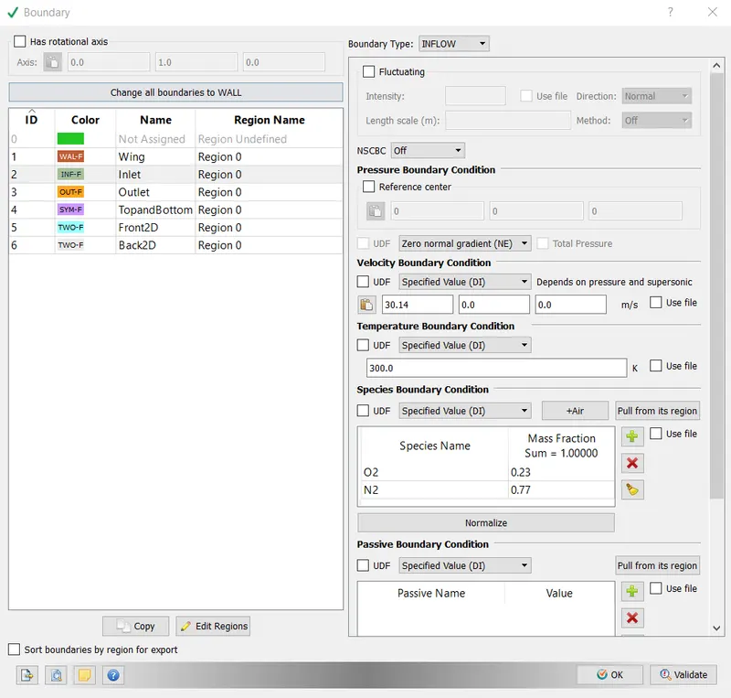
2) Inlet:

Boundary type is inflow

Pressure boundary condition: Zero normal gradient

Velocity boundary condition : Specified value(DI) =30.14 m/s in x direction.

Temperature boundary condition : Specified value = 300K

3) Outlet:

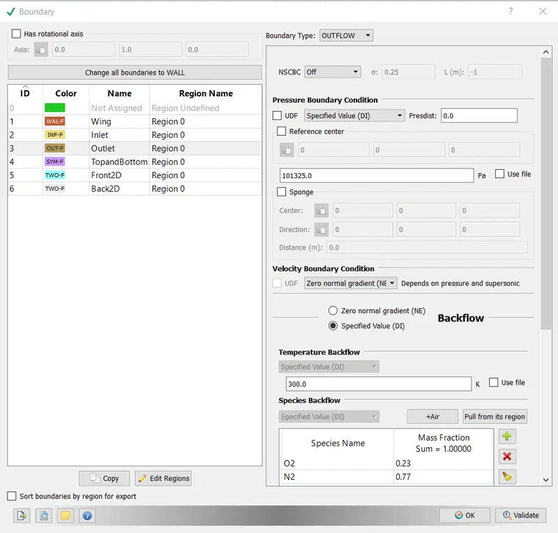
Boundary type is outflow.

Pressure boundary condition is Specified value (DI) = 101325 Pas

Velocity boundary conditioin is Zero normal gradient.

4) Top and bottom:

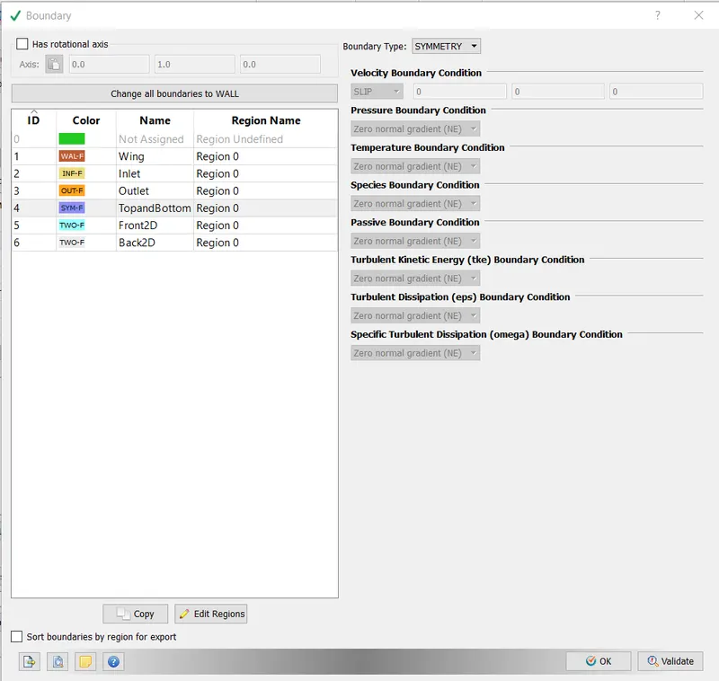
Symmetry condition prevails

Velocity boundary condition: Slip

Pressure and temperature boundary condition : Zero normal gradient.

5) Front and back 2D:

Two dimensional boundary condition prevails.

• Regions and initializations:

Region0

Stream Id =0,

veolocity is 30.14 m/s and temperature and pressure is 300K and 101325 pas.

The species dragged in are O2 and N2.

• Physical models:

Under physical model, Turbulence modelling is done only. Two turbulence models are tested, The RNG k epsilon and the standard K-omega SST modekls

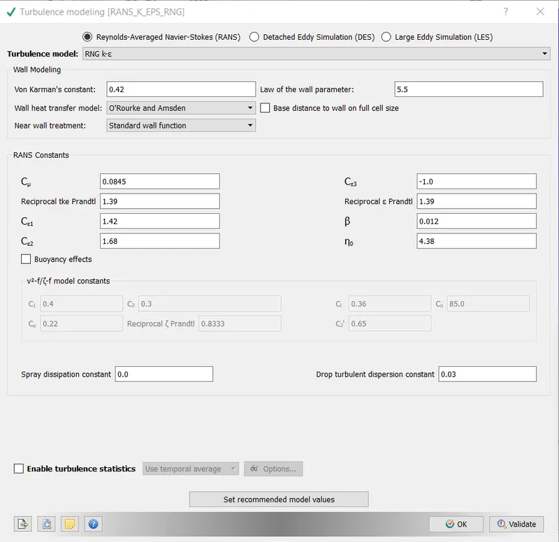
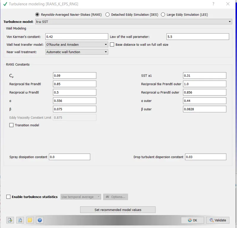
Above two turbulence models are tested for the areofoil simulation at various angle of attacks.

• Grid control:

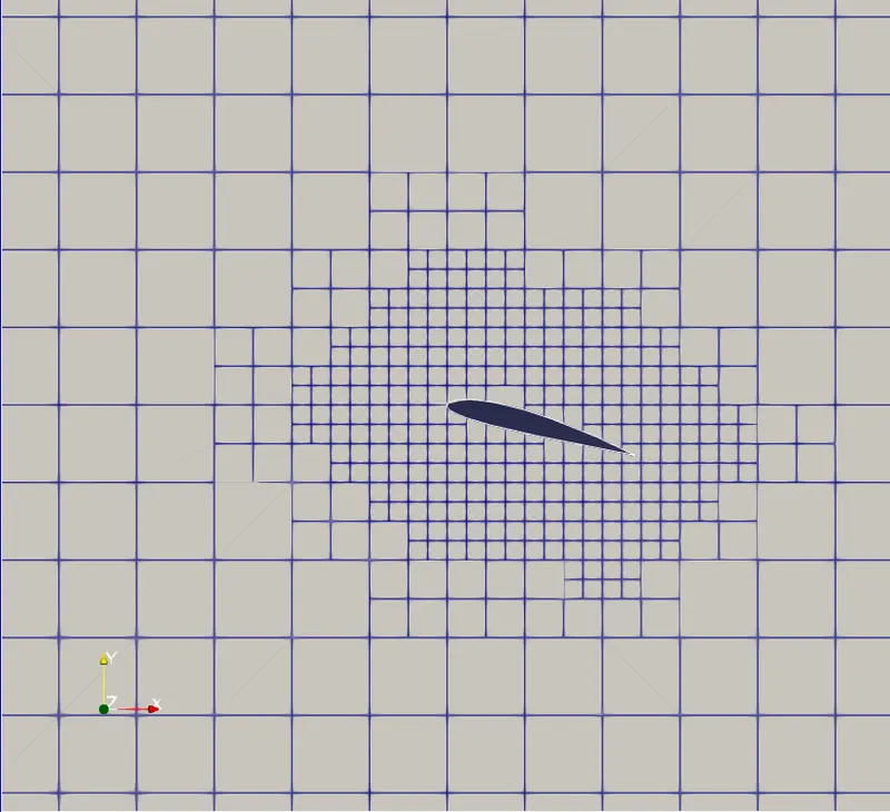
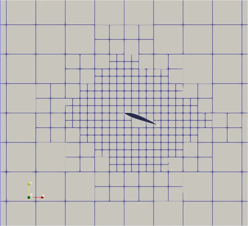
Fixed embedding box is checked.

Base grid:

dx=0.04 meters , dy=0.04 meters and dz=0.04 meters

Embedding:

Entity type : Boundary

Boundary: Wing

Mode : permanent

Scale : 2

Embedded layers : 6

• Output and post processing:

Output files:

Wall boundaries box is checked. Since this will enable to dump the wall parameters in the out put files. This is particularly important for the external aerodynamics flow simulations.

Time interval for writing output files: 0.01 seconds

Time interval for writing text files: 1e-05 seconds

Time interval for writing restart files: 0.001 seconds

Results:

The simulation is carried out four angle of attacks : 1 degree, 5 degree, 10 degree and 15 degree.

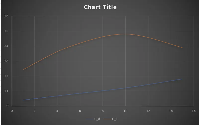
A comparative study is performed by using two turbulence models as mentioned above. the Lift and drag coefficient is calculated from the values obtained from the simulation. The Variation of drag and lift coefficient with the varying angle of attacks is put in into an chart and visualized.

Cell counts:

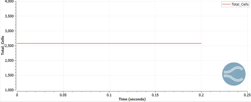
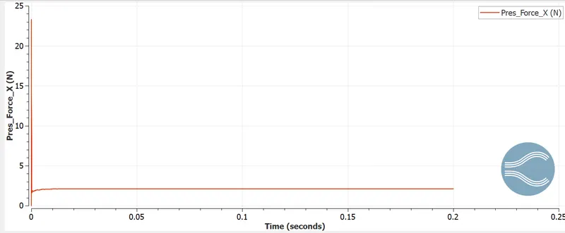
• Drag force for angle of attack 1 degree in K-omega SST model:

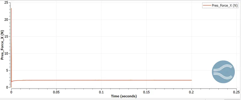
• Drag force for angle of attack 1 degree in RNG Kepsilon model:

• Drag force for angle of attack 5 degree in K omega SST model:

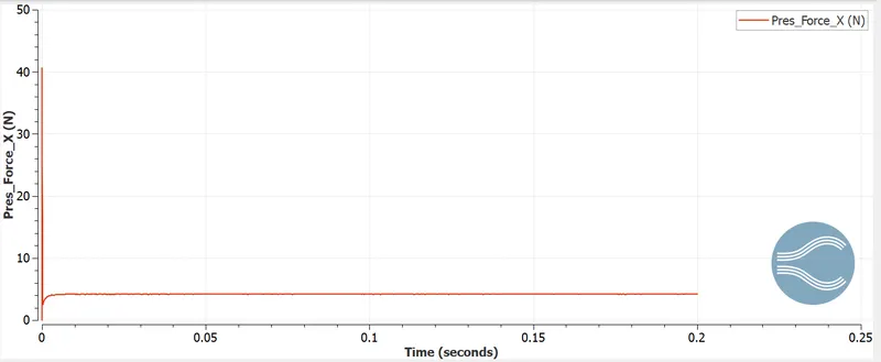
• Drag force for angle of attack 5 degree in RNG K epsilon model:

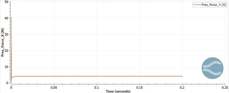
• Drag force for angle of attack 10 degrees in K omega SST model:

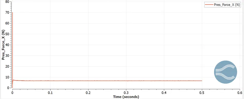
• Drag force for angle of attack 10 degrees in RNG k-epsilon model:

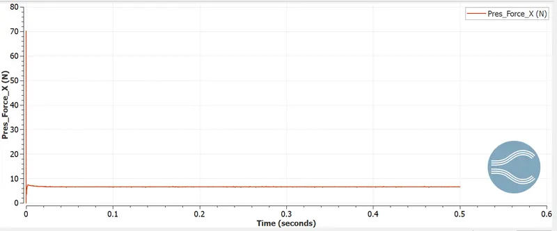
• Drag force for angle of attack 15 degrees in K omega SST model:

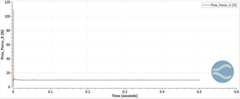
• Drag force for angle of attack 15 degrees in RNG k epsilon midel:

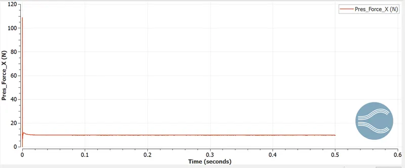
• Lift force for angle of attack 1 degree and 5 degree in K omega SST model:

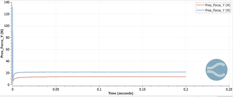
• Lift force for angle of attack 1 degree and 5 degree in RNG K epsilon model:

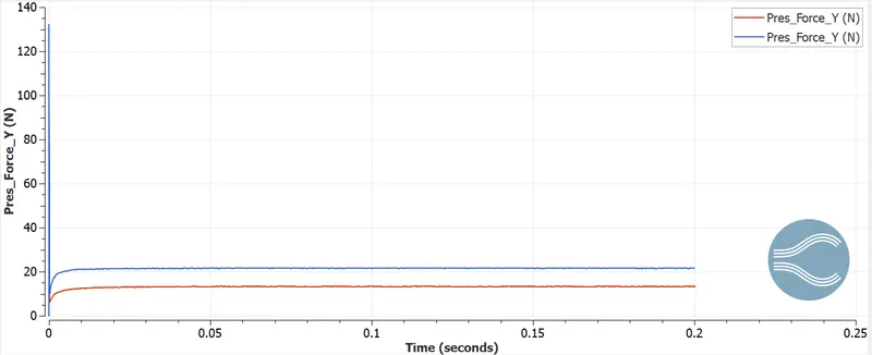
• Lift force for angle of attack 10 degree and 15 degree in K omega SST model:

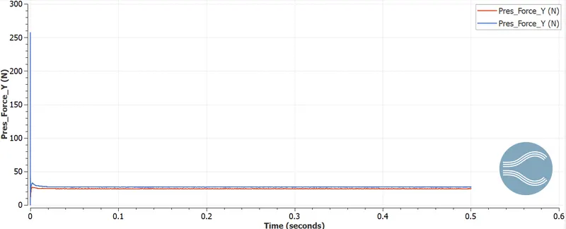
• Lift force for angle of attack 10 degree and 15 degree in RNG K -epsilon model:

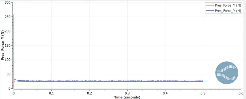
Calculation of drag and lift coefficient:

Angle of attack	Turbulence model	Drag force	Lift force	Drag coefficient	Lift coefficient
1	K-omega SST	2.11393	13.3786	0.0386	0.2431
1	RNG K epsilon	2.11429	13.3234	0.0300	0.2448
5	K-omega SST	4.21886	21.5473	0.077	0.3900
5	RNG K epsilon	4.18531	21.5517	0.076	0.3939
10	K Omega SST	6.55044	24.4601	0.1298	0.4801
10	RNG K epsilon	6.59676	24.5970	0.1200	0.4800
15	K Omega SST	9.91812	19.8199	0.1878	0.3901
15	RNG K epsilon	9.80275	19.6801	0.1865	0.3976

`C_d=(F_d)/(0.5*rho*V^2*A)` here A is the frontal projection area = 0.1 m^2

Whwn the drag coefficient and lift coefficient is plotted against the angle of attacks :

Discussion of the result:

• The coefficient of lift increases with the increase in the angle of the attack. After a certain angle of attack, the coefficient of lift decreases. This phenomenon is called stalling condition.
• The dip in the lift force is due to the vortex formation in the leeward side of the aerofoil.
• in case of the drag force, the pressure drag component in the total drag is very less in case of the aerofoil till 10 degrees angle of attack. After the 10 degree angle of attack, the pressure drag increases significantly , due to the vortex formation. So the total drag increases.

• Average Y-plus value:

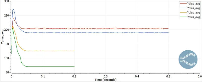
the average y plus value for the angle of attacks increases with the increase in the angle of attack.

y+ is a non-dimensional distance. It is often used to describe how coarse or fine a mesh is for a particular flow pattern. It is important in turbulence modeling to determine the proper size of the cells near domain walls.

The average value of the Y+ is between 30 and 300. In these cases the Y+ is much inside the limits.

Post processing:

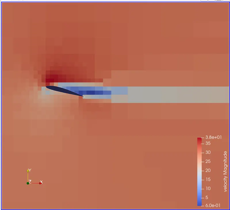
• velocity contour:

Angle of attack = 10 degree

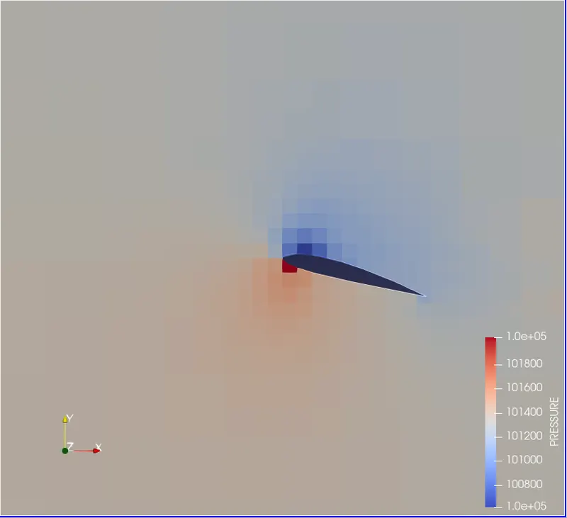
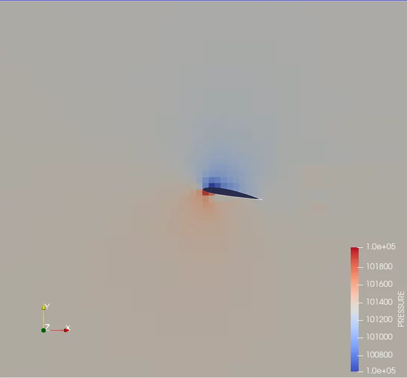
• Pressure contour :

• Mesh generation:

• Angle of attack = 15 degrees

1) Mesh generation:

2) Velocity contour:

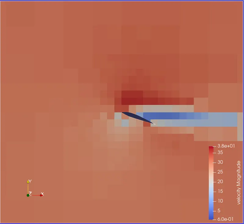
3) Pressure contour:

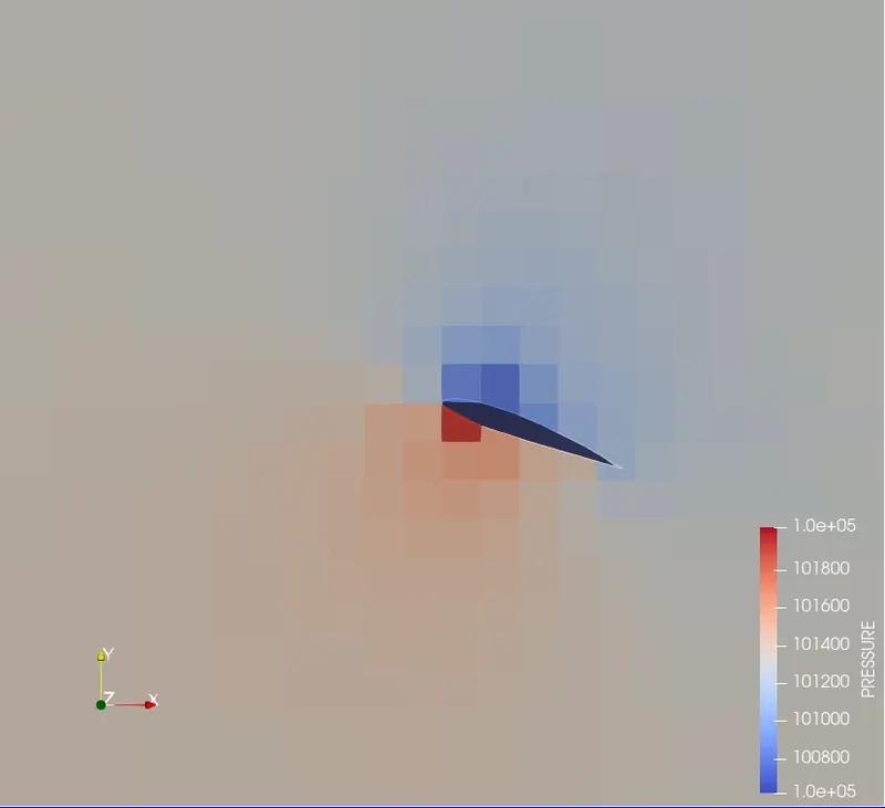
• Angle of attack 5 degree:

1) Mesh generation 2) velocity contour 3) Pressure contour

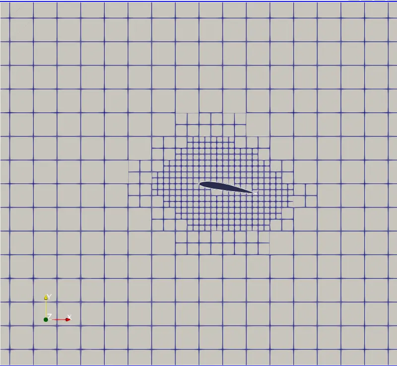
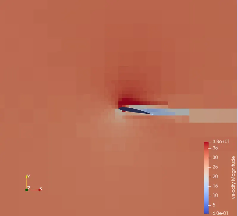
Animation :

velocity contour animation : https://youtu.be/n5hY949fVAY

Pressure contour animation: https://youtu.be/8jcaN3A3uHc

• From all the contours of pressure , it can be seen that the pressure at the upper side is lower than that of the lower side , that generates the lift.

Conclusion:

• The flow over NACA 2412 aerofoil is done for various angle of attacks
• The two turbulence mod3l is used in the simulation. A comparative study is done between the two.
• Velocity and pressure variation across the aerofoil is done.