Week 9 - Mini project - Flow over an Airfoil

Week 9 - Mini project - Flow over an Airfoil

Aim:

To simulate flow over a 4 digit airfoil i.e NACA 2412 Airfoil.

To calculate the following,

• Drag co-efficient Vs Angle of Attack
• Lift co-efficient vs Angle of Attack
• Compare the effect of turbulence models on the above two results.
• Make sure that the inlet Reynolds number is 200,000
• Make sure you do above calculations for the following angle of attacks,
  1. Angle of attack = 1º
  2. Angle of attack = 5º
  3. Angle of attack = 10º
  4. Angle of attack = 15º

Introduction:

Airfoil:

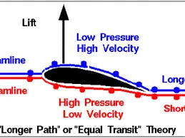
The cross-sectional shape of wing is called an Airfoil. The airfoil is primarily responsible to generate lift force which acts perpendicular to the direction of the airflow. Lift force is created because of the pressure difference between the upper and the lower surface of the airfoil. On the upper surface of the airfoil the flow is slower than the flow in the lower surface, so the air pressure over the top surface of the airfoil is less than the pressure in the bottom surface. This causes the airfoil to encounter lift force. The lift depends on the shape of the airfoil, velocity, density of air, surface area and angle of attack of the airfoil.

Aerodynamic forces are produced when a solid body passes through the fluid body. By modifying the geometry of the airfoil, it can be used for various applications and at different speed. In case of subsonic flight condition, rounded leading edge condition is used and for supersonic condition a sharp leading-edge condition of the airfoil is used.

The angle of attack of the airfoil plays an important role in producing lift. The oncoming air is deflected when the angle of attack is fixed with certain angle of attack which results in force on the airfoil in the direction opposite to the deflection. The main two forces acting on an airfoil is lift and drag. Most airfoil shape requires a positive angle of attack to generate lift. In case of cambered airfoils, it can produce lift at zero angle of attack because of its geometric properties.

Airfoil terms and definitions:

Leading edge: The section of the airfoil which hits the air first.

Trailing edge: Section of the airfoil which hits the air last.

Chord: The distance between the leading edge and trailing edge.

Chord Line: A straight line joining the leading edge and the trailing edge.

Camber line: Line joining the leading edge and trailing edge that is equidistant from the top and bottom surfaces.

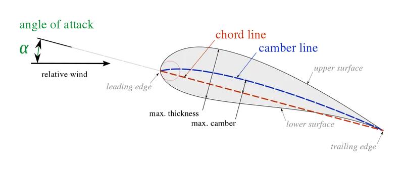
Camber: Distance from the camber line to the chord line.

Thickness: Distance from the top surface to the bottom surface.

Leading Edge Radius: Radius of curvature at the leading edge.

Pitching moment: The torque or twisting force created on airfoil by the aerodynamic forces acting on it.

Centre of Pressure: A point on the airfoil where the resultant lift vector can be considered to be acting at a point where the pitching moment is zero.

Aerodynamic center: Pitching moment is independent of the angle of attack and lift co-efficient.

Angle of attack: Angle between the relative wind and the chord line. Increase in angle of attack results in an increase in the lift.

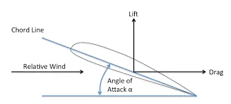
Stall: Lift suddenly decreases and the drag increases because of the increase in the angle of attack.

Stall angle: Angle of attack at which the stall occurs.

Thickness: It varies along the chord. It can be measured in either of the following two methods.

1. Thickness measured perpendicular to the camber line.
2. Thickness measured perpendicular to the chord line.

Airfoil Types:

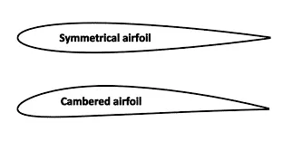
There are essentially two types of aerofoils- symmetrical and non-symmetrical. Symmetrical aerofoil has identical upper and lower surfaces such that the chord line and mean camber line happen to be the same, resulting in the production of no life at zero AOA. Moreover, this type has application in the main rotor blades of various light helicopters.

Non-symmetrical aerofoil, also known as cambered aerofoil, has different upper and lower surfaces such that the chord line happens to be placed above with large curvature. Furthermore, their chord line and chamber line are different. Also, the advantages of this type are a better lift to drag ratio and stall characteristics, thereby resulting in the production of a useful lift at zero AOA.

Drag:

It is the common force that a body meets some resistance when it is forced to move through a fluid. We could notice that we feel difficult to walk in water because of the much greater resistance it offers to motion compared to air. A fluid may exert forces and moments on a body in and about various directions. The force a flowing fluid exerts on a body in the flow direction is called drag. The drag forces can be measured directly by simply attaching the body subjected to fluid flow to a calibrated spring and measuring the displacement in the flow direction experimentally. The most researches have been centred around the reduction of drag. Reduction of drag is closely associated with the reduction of fuel consumption in automobiles. But in certain cases, drag produces a beneficial effect and we try to maximize it.

Drag force is proportional to the velocity for low-speed flow and the squared velocity for high-speed flow, where the distinction between low and high speed is measured by the Reynolds number. Drag forces always tend to decrease fluid velocity relative to the solid object in the fluid's path.

The drag depends on the density of the fluid, the upstream velocity, size, shape of the body. The drag co-efficient is calculated by using the following formula.

`F_D=1/2 *rho*v^2*C_D*A`

where

`F_D` is the drag force

`rho` is the density of the fluid

`v` is the velocity of the fluid

`A` is the cross sectional area

`C_D` is the drag co-efficient.

Lift:

A fluid flowing around an object exerts a force on it. Lift is the component of this force that is perpendicular to the oncoming flow direction. It contrasts with the drag force, which is the component of the force parallel to the flow direction. Lift conventionally acts in an upward direction in order to counter the force of gravity, but it can act in any direction at right angles to the flow.

The lift co-efficient is calculated by using the following formula.

`F_L=1/2*rho*v^2*C_L*A`

where

`F_L` is the lift force

`rho` is the density of the fluid

`v` is the velocity of the fluid

`A` is the cross sectional area

`C_L` is the lift co-efficient.

NACA Airfoil:

The NACA airfoils are airfoil shapes for aircraft wings developed by the National Advisory Committee for Aeronautics (NACA). The shape of the NACA airfoils is described using a series of digits following the word "NACA". The parameters in the numerical code can be entered into equations to precisely generate the cross-section of the airfoil and calculate its properties.

The NACA four-digit wing sections define the profile by:

• First digit describing maximum camber as percentage of the chord.
• Second digit describing the distance of maximum camber from the airfoil leading edge in tenths of the chord.
• Last two digits describing maximum thickness of the airfoil as percent of the chord.

The NACA 2412 airfoil has a maximum camber of 2% located 40% (0.4 chords) from the leading edge with a maximum thickness of 12% of the chord.

Geometry Setup:

• NACA 2412 Airfoil’s co-ordinates are added to the geometry by using the following command. Geometry --> Create --> Vertex --> Add the co-ordinates one by one from the available co-ordinates --> Apply.

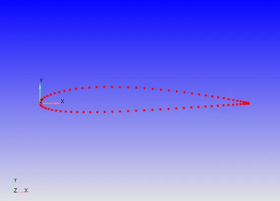
• The vertices are stitched together to form triangles by using the following step. Geometry --> Repair --> Patch --> Ordered Vertex list --> Select the vertices --> Apply. The chord length of the airfoil is scaled to be 0.1 m.

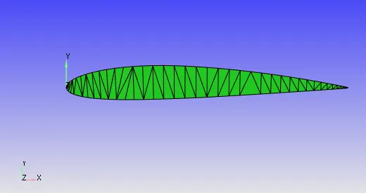
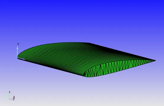
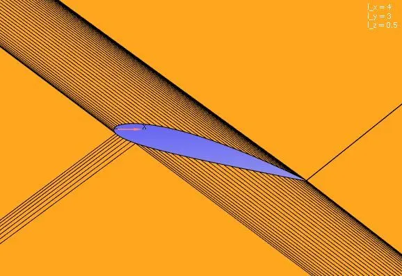
• Once the airfoil’s geometry is created a virtual wind tunnel was also made for setting up the simulation. The length from the leading edge to the inlet section of the wind tunnel is set to 2.0 m and the distance from the leading edge to the outlet section of the wind tunnel is set to 2.0 m. The total height of the wind tunnel is 3 m. Since this is 2D simulation the length of the wind tunnel across the Z-direction is not much of importance and hence an appropriate length can be given.

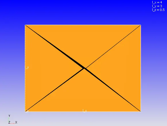
• Diagnosis toolbar is used for geometry check-up.

• In converge every part of the geometry is assumed to be triangle. The group of triangles are assigned to form a boundary. The boundaries are formed by using the following command. Geometry --> Boundary --> Flag --> Add boundary --> Create two boundaries --> Select the particular triangles and allot them to one region --> Apply.

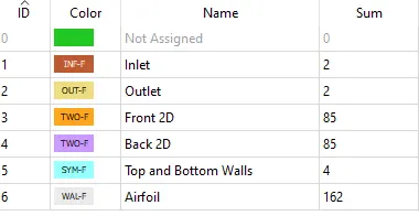
• Then the normal are checked whether they are pointing inside the geometry where does the flow passes.

Case Setup:

• The application type is fixed with time based.
• Then click on Materials which is present in the right side of the window that is case setup tree and select the Predefined mixtures as Air.

i) Materials:

• Click on the Gas simulation and Global Transport parameter and retain the same values.
• Click on Species and then add O2 and N2.

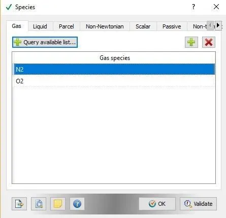
ii) Simulation Parameters:

• Click on Run Parameters and under the solver tab choose the solver as Steady-State Solver. Set the simulation mode to Full Hydrodynamic and the gas flow solver as compressible.
• Since this is a transient simulation case setup, end time was calculated using the flow through time formula. Flow through time is the time taken by the fluid particles to travel from the inlet to outlet boundary with certain inlet velocity. In order to estimate the time taken, inlet velocity was calculated based on the given Reynolds number.

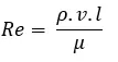
Re = 200000

Characteristic length of the airfoil, l = 0.1 m

At 300K, following parameters of air are used,

`rho` = 1.1765 kg/`m^3`

`mu=1.8538*10^-5 (kg)/(m*s)`

`v` = 31.51 m/s

Using the calculated inlet velocity, the flow through was calculated using the following formula.

Flow through time = Total Length of the wind Tunnel / Inlet Velocity

Therefore, Flow through time = `4/31.51`

Flow though time is approximately = 0.12 seconds.

As a best practice in transient flow simulation, the flow has to pass 4 times through the geometry.

Hence the end time was set with 4*0.12 = 0.48 seconds.

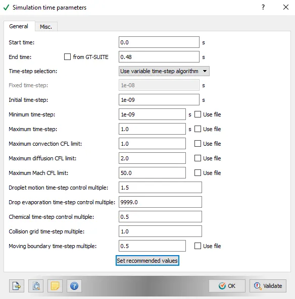
• Then under Solver Parameters retain the default settings.

iii) Initial Conditions and Events:

Regions and Initialisation:

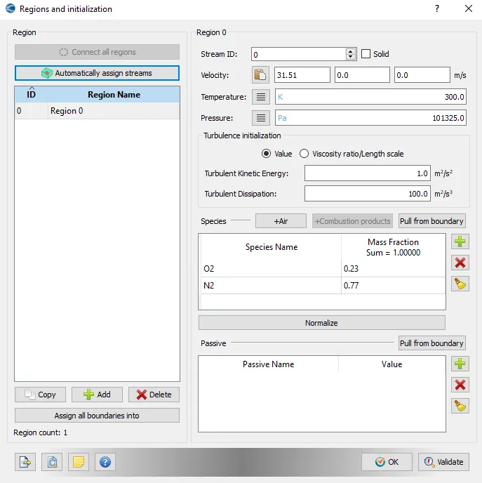
• Grouping the boundaries to form volumetric zones called region. This defines a volumetric region with initial conditions like initial pressure, initial temperature, velocity and species concentration.

• Under Regions and Initialisation, select add to create regions. Add a region and assign the velocity to be 31.51 m/s in X-direction. Add the species.

iv) Boundary Conditions:

Boundary:

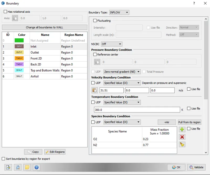
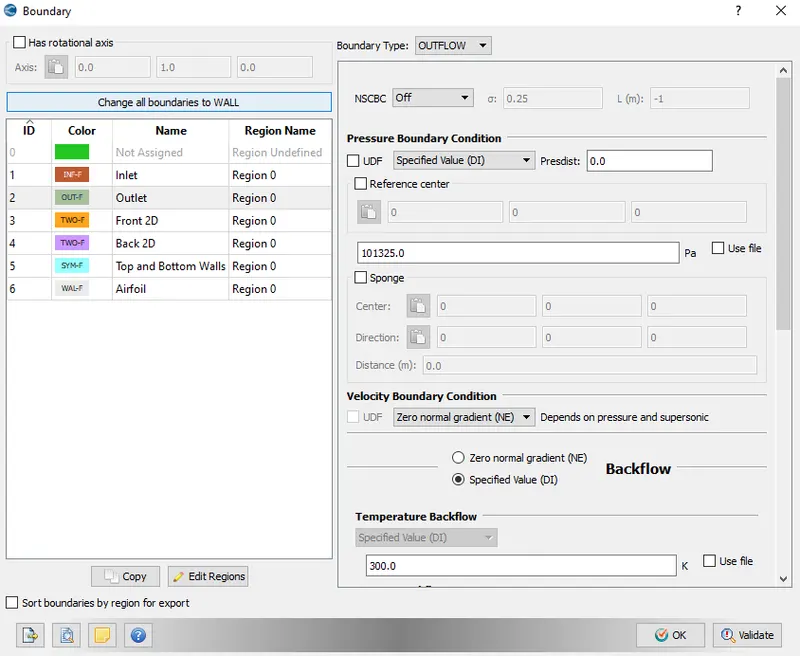
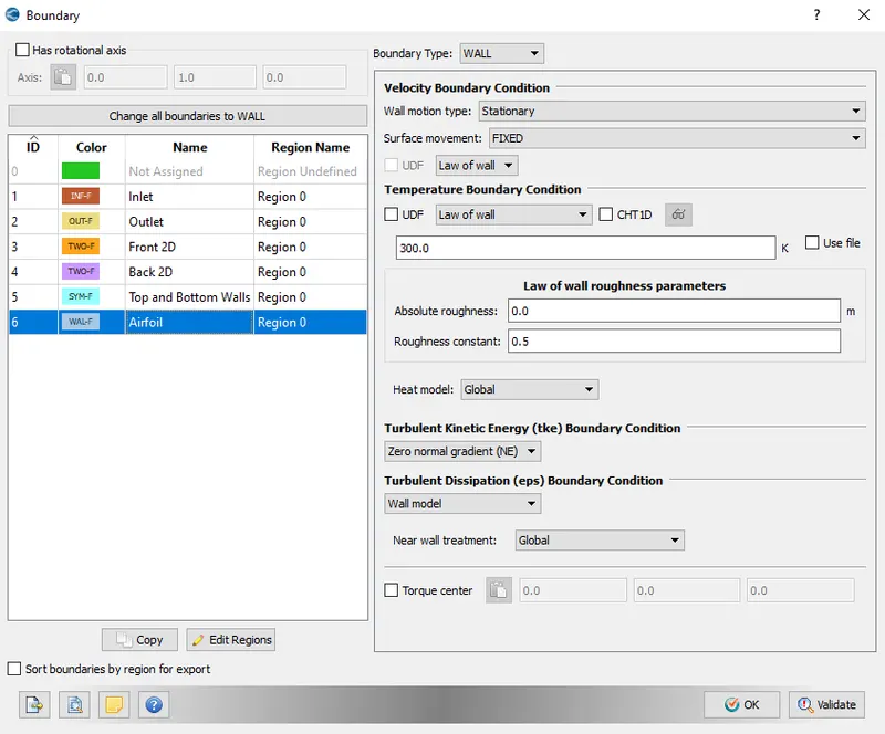
Under this parameter the boundaries have been defined and assigned with the following boundary conditions.

Inlet:

Outlet:

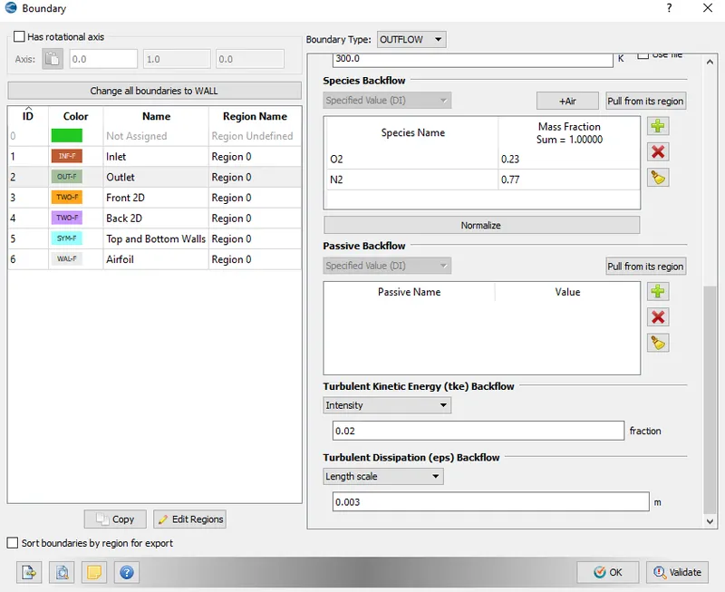
Both the Front 2D and Back 2D is assigned with TWO_D boundary type. The Top and Bottom Walls boundary is assigned with Symmetry boundary type.

Airfoil:

v) Physical Models:

Turbulence Modelling:

Then under the physical models check the turbulence modelling and set with Reynolds Averaged Navier-Stokes (RANS) and set the turbulence model with RNG K-epsilon and K-omega SST model.

vi) Grid Control:

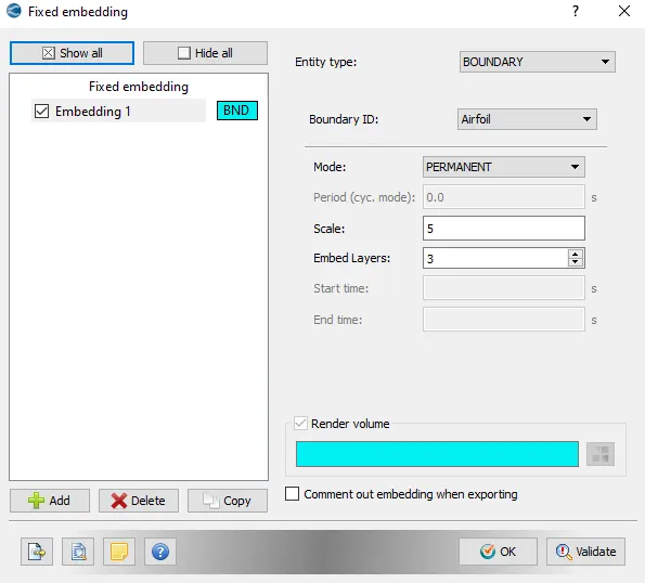
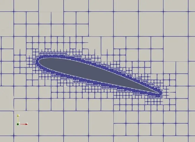
Under grid control tab enable the Fixed Embedding option.

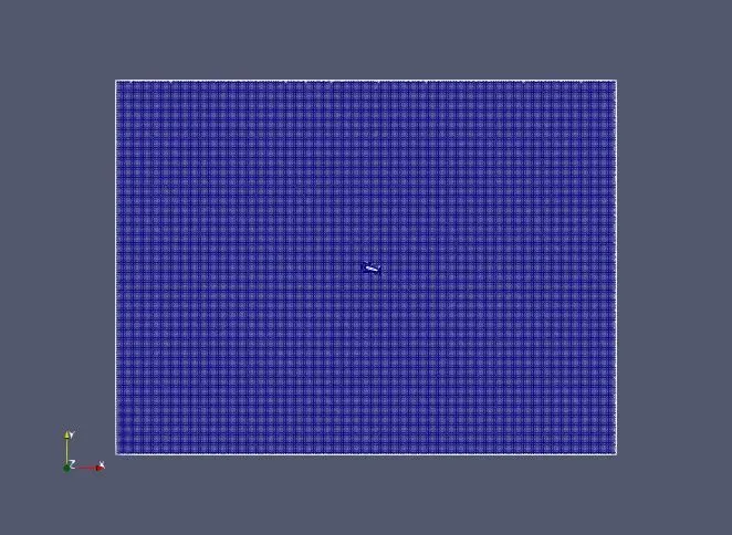
Then in the Grid Control parameter --> Base Grid --> Enter the size of the grid.

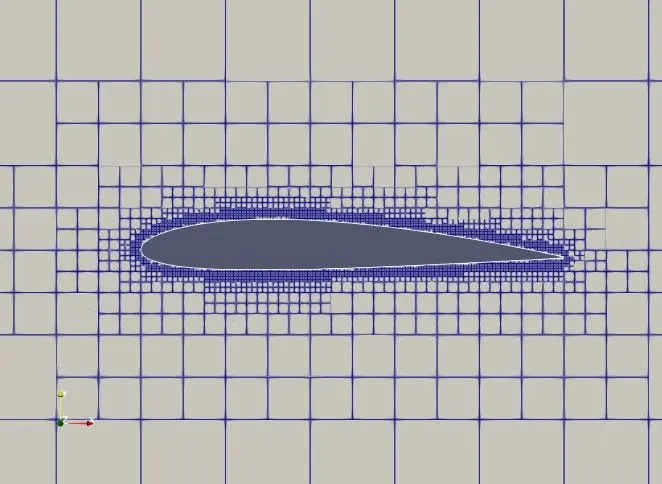
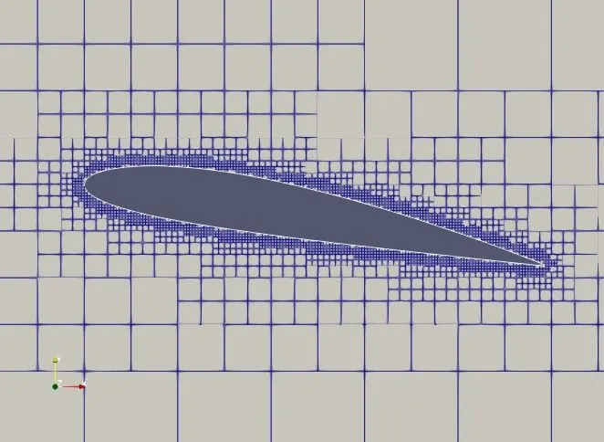
The size of the grid is assigned with 0.02 m. In order to have a correct approximation near the wall of the airfoil, fixed embedding parameter was used for the entire simulation time. The fixed embedding scale is important to observe the turbulence and flow separation near the airfoil wall. As we are using RNG K-epsilon model the y+ value should be greater than 30. In this project we have used the y+ value of 50 and calculated the first layer thickness and the scale value for fixed embedding.

vii) Output/Post-Processing:

Then under Output/Post-Processing --> Post Variable Selection --> Under Combustion/Turbulence enable the y+ parameter and add the Mass fraction with O2 and N2

Then under the Output files --> Writing time intervals --> set the time interval for writing 3D output data files and time interval for writing restarting output.

Then use CYGWIN to execute the CFD solver.

Then with the help of Converge CFD the post converting the output files to Paraview format is done.

Paraview is used for Post processing the results.

Results:

Case 1:

Solver: RNG k-epsilon

Angle of Attack = 1 degree

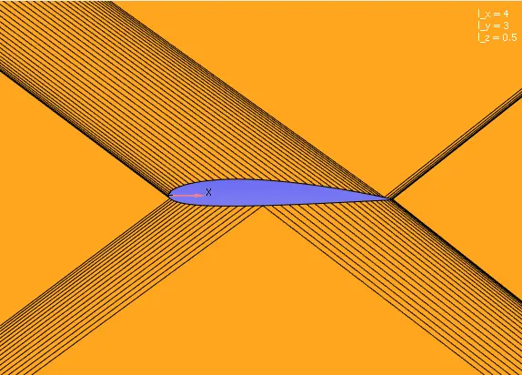
Geometry:

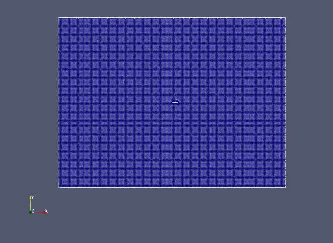
Mesh:

Velocity contour:

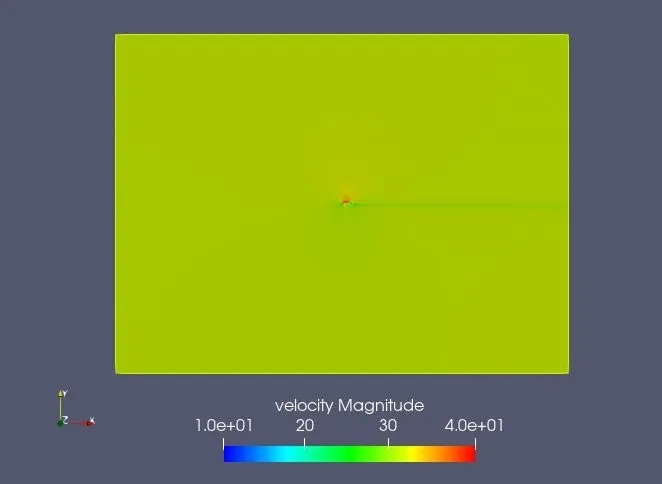
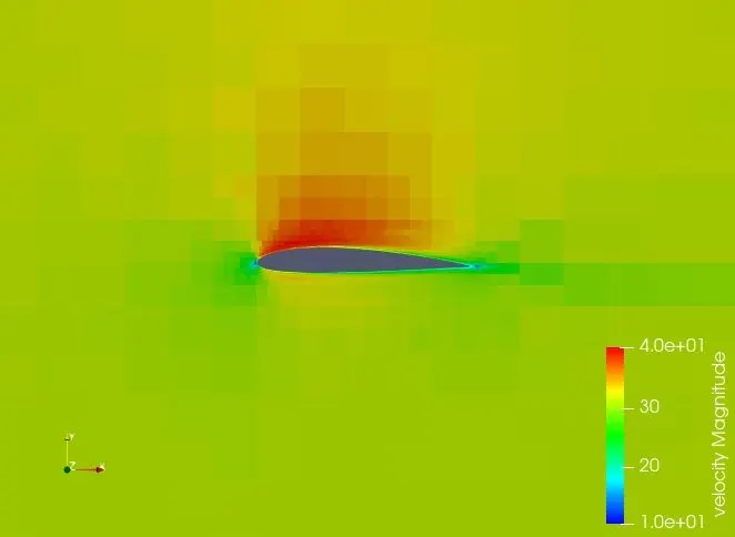
From the above contour plot we could observe that the velocity is clearly high on the upper surface of the airfoil and the velocity is lesser on the lower side of the airfoil. This is because of the airfoil geometry where the upper surface have a negative slope (curved downwards) where the air-molecules can move down easily and they also have their internal kinetic energy which increasess the velocity.

Pressure Contour:

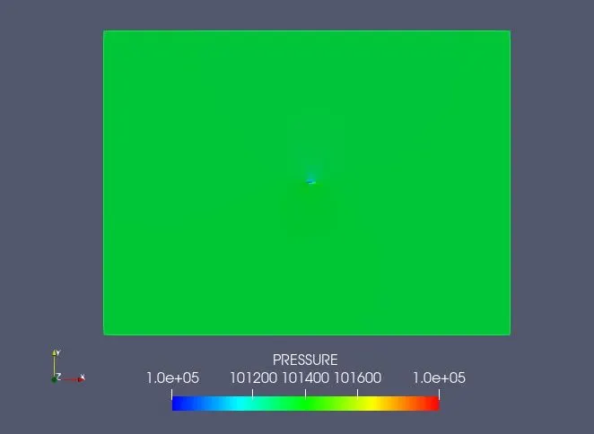
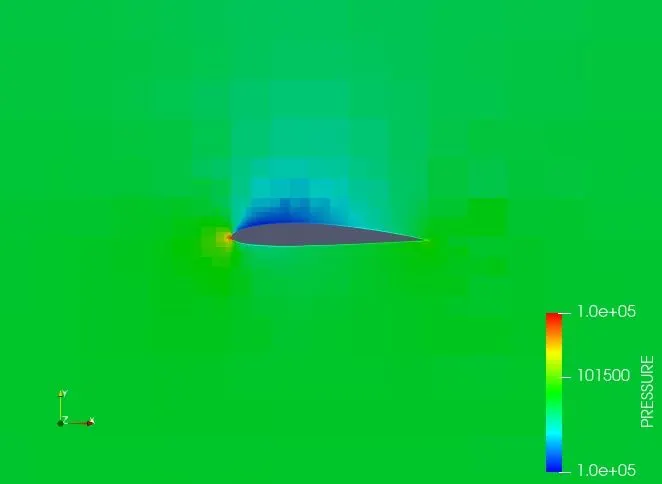
From the above contour plots we could predict that a low pressure region is created on the top of the airfoil because of its shape and velocity of the fluid.

Outlet Velocity:

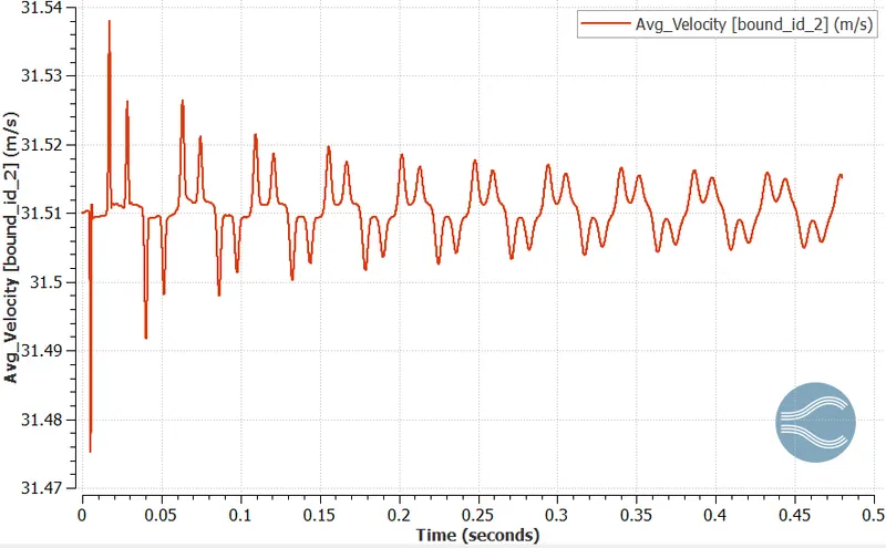
Pressure_Force_X (N):

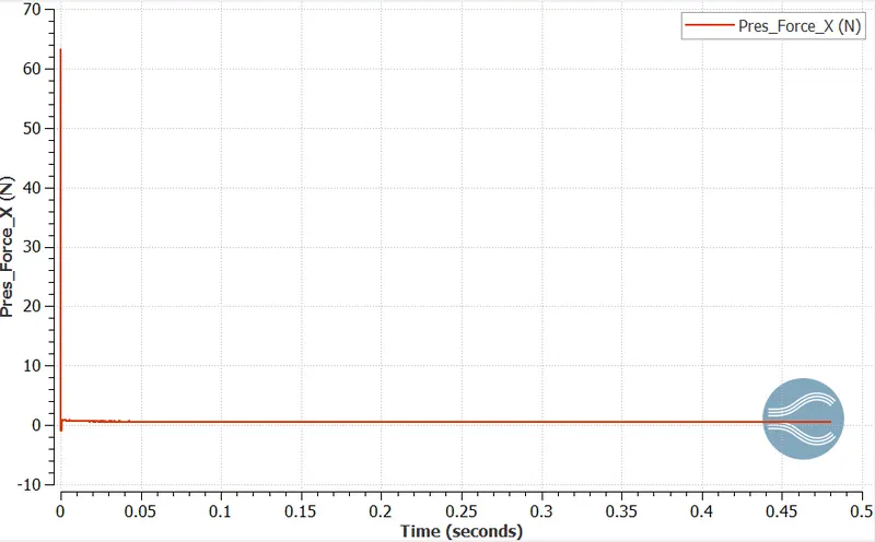
The above graph represents the pressure force in x-direction which is nothing but the drag produced by the airfoil body at a free stream velocity of 31.51 m/s

Pressure_Force_Y (N):

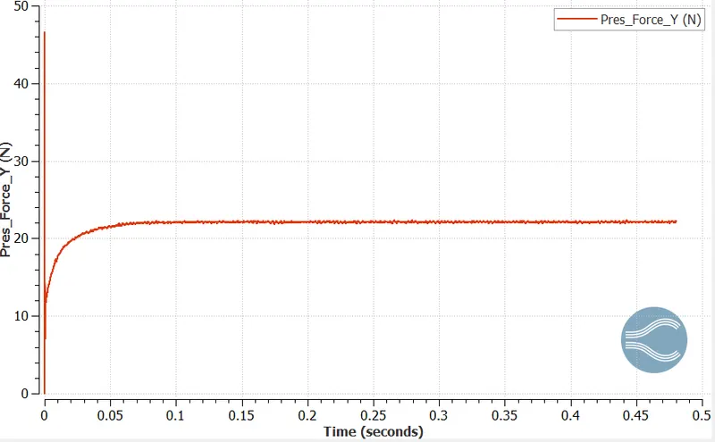
The above graph represents the pressure force in y-direction which is nothing but the lift produced by the airfoil body at a free stream velocity of 31.51 m/s

Hence from the above plots we could attain the value of drag and lift forces which can be used for calculating the co-efficient of drag and lift.

`F_D=0.535643`

`F_L=22.095`

`rho=1.1765(kg)/m^3`

`A=0.1`

`v=31.51 m/s`

Drag Calculation:

`C_D=(2*F_D)/(rho*v^2* A)`

`C_D = (2*0.535643)/(1.1765*31.51^2*0.1)`

`therefore C_D=0.0091709`

Lift Calculation:

`C_L=(2*F_L)/(rho*v^2* A)`

`C_L = (2*22.095)/(1.1765*31.51^2*0.1)`

`therefore C_L =0.37829`

Case 2:

Solver: RNG k-epsilon

Angle of Attack = 5 degree

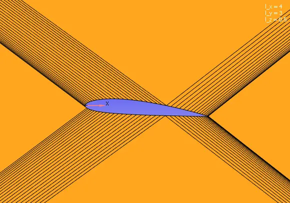
Geometry:

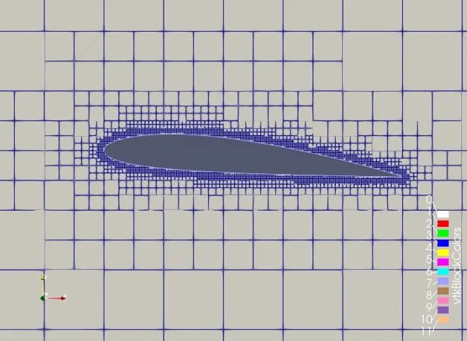
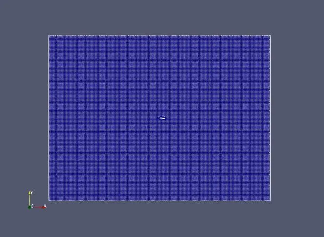
Mesh:

Velocity Contour:

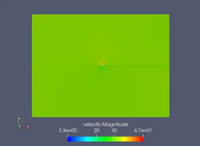
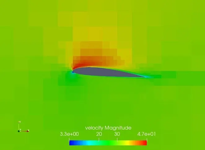
From the above contour plot we could observe that the velocity is clearly high on the upper surface of the airfoil and the velocity is lesser on the lower side of the airfoil. This is because of the airfoil geometry where the upper surface have a negative slope (curved downwards) where the air-molecules can move down easily and they also have their internal kinetic energy which increasess the velocity.

Pressure Contour:

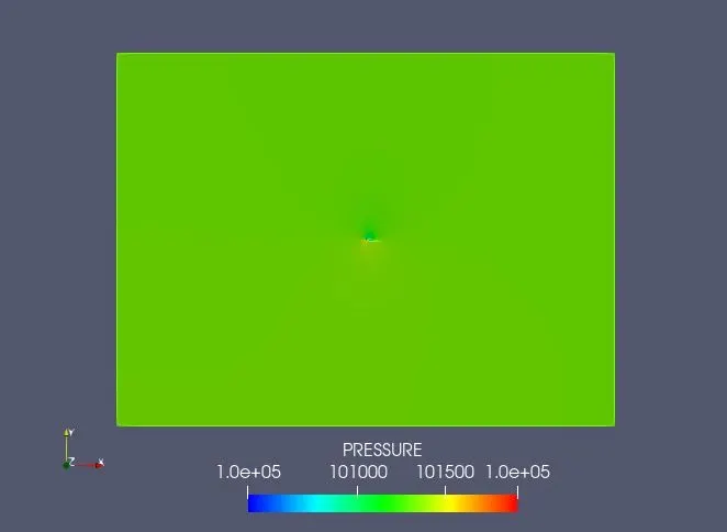
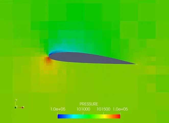
From the above contour plots we could predict that a low pressure region is created on the top of the airfoil because of its shape and velocity of the fluid.

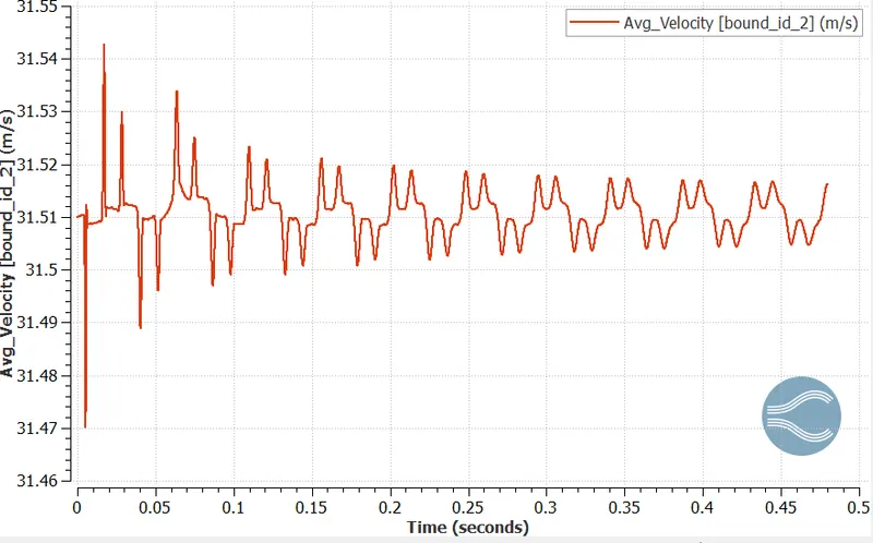
Outlet Velocity:

Pressure_Force_X (N):

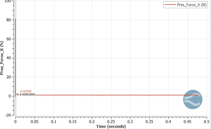
The above graph represents the pressure force in x-direction which is nothing but the drag produced by the airfoil body at a free stream velocity of 31.51 m/s

Pressure_Force_Y (N):

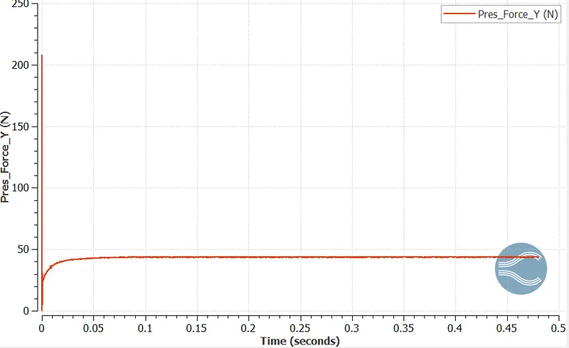
The above graph represents the pressure force in y-direction which is nothing but the lift produced by the airfoil body at a free stream velocity of 31.51 m/s

Hence from the above plots we could attain the value of drag and lift forces which can be used for calculating the co-efficient of drag and lift.

`F_D=0.9777085`

`F_L=43.6845`

`rho=1.1765(kg)/m^3`

`A=0.1`

`v=31.51 m/s`

Drag Calculation:

`C_D=(2*F_D)/(rho*v^2* A)`

`C_D = (2*0.977085)/(1.1765*31.51^2*0.1)`

`therefore C_D=0.016729`

Lift Calculation:

`C_L=(2*F_L)/(rho*v^2* A)`

`C_L = (2*43.6845)/(1.1765*31.51^2*0.1)`

`therefore C_L=0.74794`

Case 3:

Solver: RNG k-epsilon

Angle of Attack = 10 degree

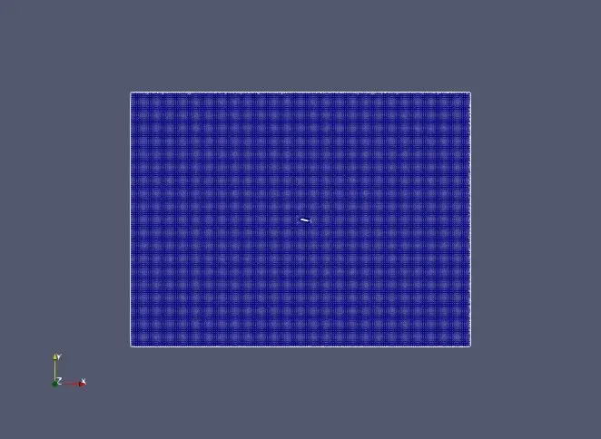
Geometry:

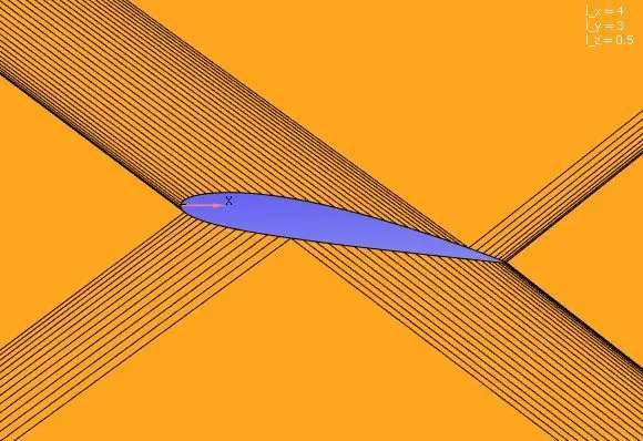
Mesh:

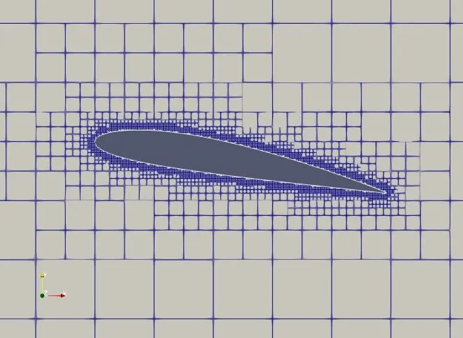
Velocity Contour:

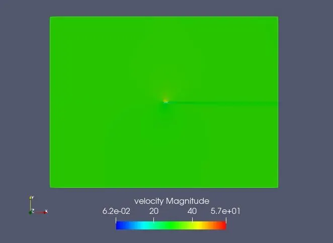
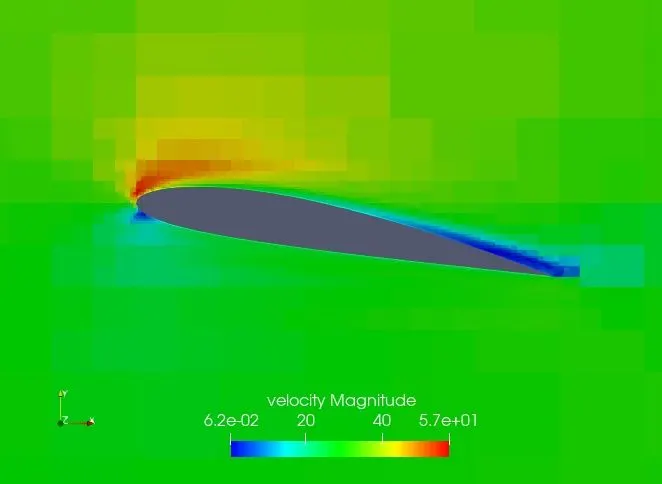
From the above contour plot we could observe that the velocity is clearly high on the upper surface of the airfoil and the velocity is lesser on the lower side of the airfoil. This is because of the airfoil geometry where the upper surface have a negative slope (curved downwards) where the air-molecules can move down easily and they also have their internal kinetic energy which increasess the velocity.

Pressure Contour:

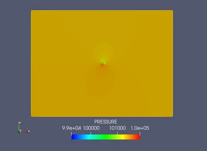
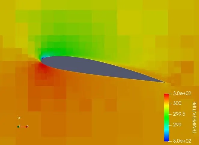
From the above contour plots we could predict that a low pressure region is created on the top of the airfoil because of its shape and velocity of the fluid.

Outlet Velocity:

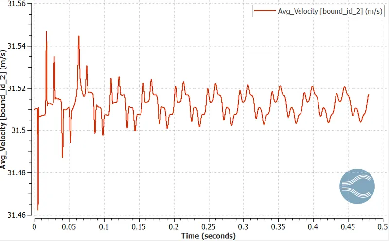
Pressure_Force_X (N):

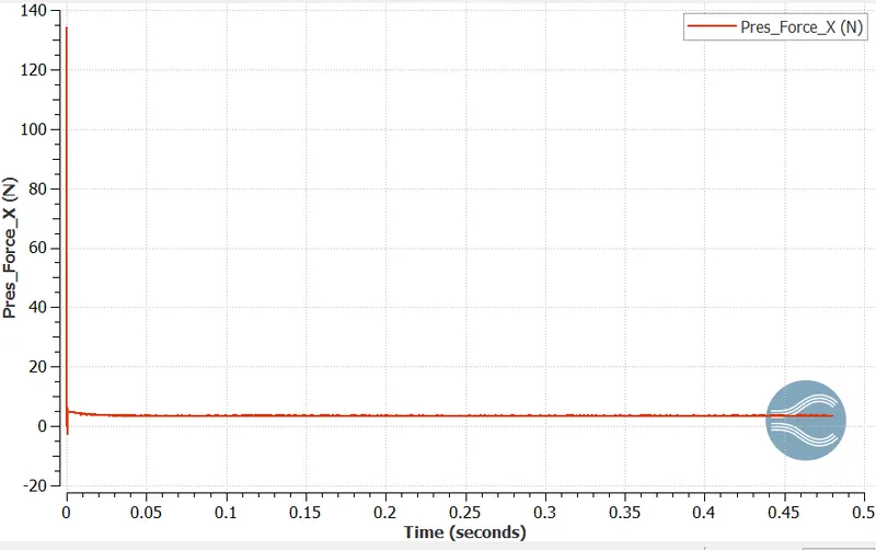
The above graph represents the pressure force in x-direction which is nothing but the drag produced by the airfoil body at a free stream velocity of 31.51 m/s

Pressure_Force_Y (N):

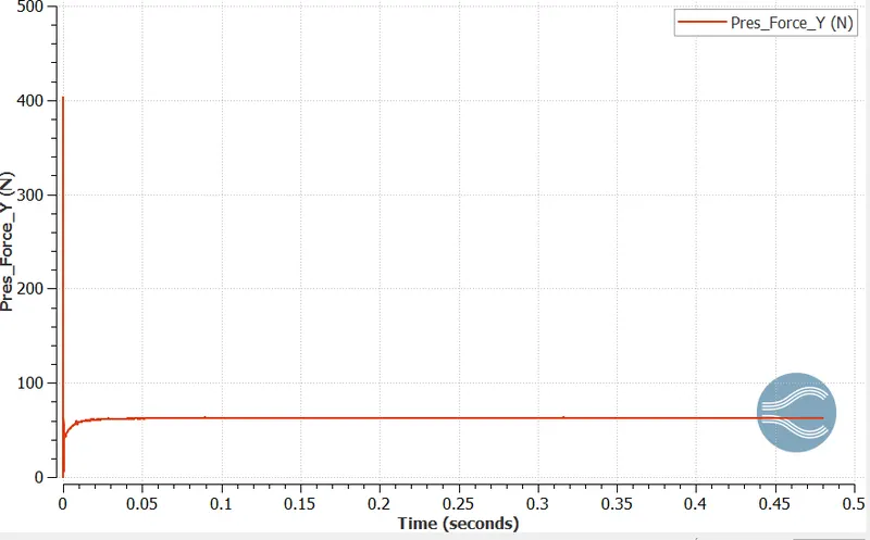
The above graph represents the pressure force in y-direction which is nothing but the lift produced by the airfoil body at a free stream velocity of 31.51 m/s

Hence from the above plots we could attain the value of drag and lift forces which can be used for calculating the co-efficient of drag and lift.

`F_D=3.44024`

`F_L=62.7915`

`rho=1.1765(kg)/m^3`

`A=0.1`

`v=31.51 m/s`

Drag Calculation:

`C_D=(2*F_D)/(rho*v^2* A)`

`C_D = (2*3.44024)/(1.1765*31.51^2*0.1)`

`therefore C_D=0.05890`

Lift Calculation:

`C_L=(2*F_L)/(rho*v^2* A)`

`C_L = (2*62.7915)/(1.1765*31.51^2*0.1)`

`therefore C_L=1.0750`

Case 4:

Solver: RNG k-epsilon

Angle of Attack = 15 degree

Geometry:

Mesh:

Velocity Contour:

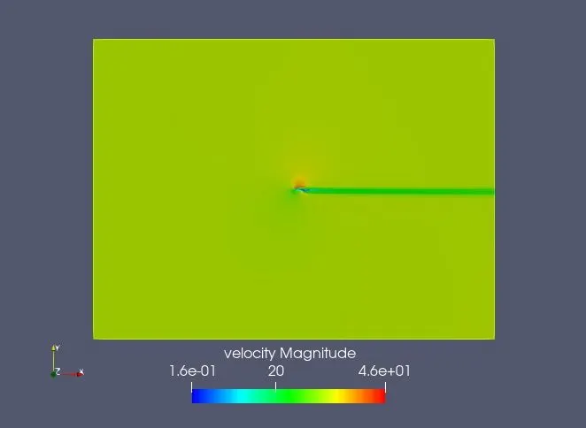
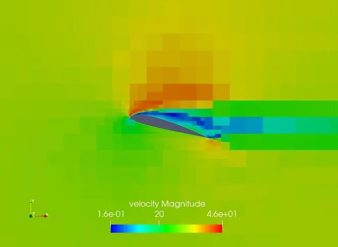
From the above contour plot we could observe that the velocity is clearly high on the upper surface of the airfoil and the velocity is lesser on the lower side of the airfoil. This is because of the airfoil geometry where the upper surface have a negative slope (curved downwards) where the air-molecules can move down easily and they also have their internal kinetic energy which increasess the velocity.

Pressure Contour:

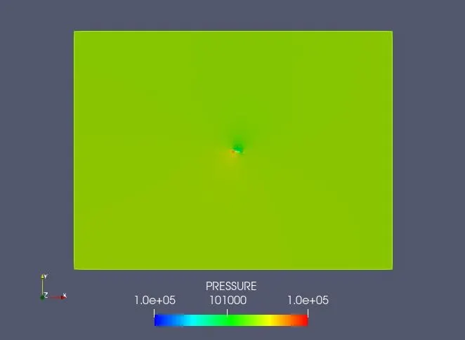
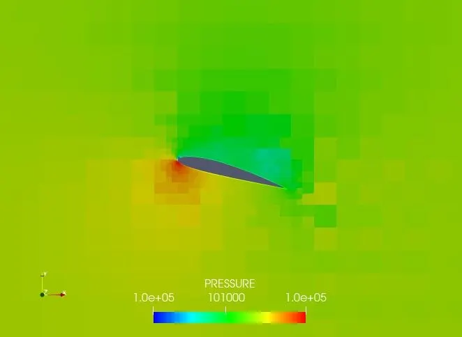
From the above contour plots we could predict that a low pressure region is created on the top of the airfoil because of its shape and velocity of the fluid.

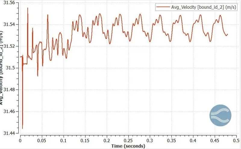
Outlet Velocity:

Pressure_Force_X (N):

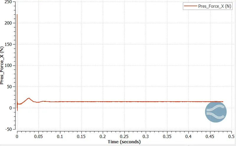
The above graph represents the pressure force in x-direction which is nothing but the drag produced by the airfoil body at a free stream velocity of 31.51 m/s

Pressure_Force_Y (N):

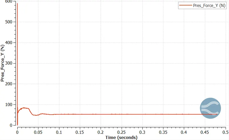
The above graph represents the pressure force in y-direction which is nothing but the lift produced by the airfoil body at a free stream velocity of 31.51 m/s

Hence from the above plots we could attain the value of drag and lift forces which can be used for calculating the co-efficient of drag and lift.

`F_D=14.7939`

`F_L=52.9155`

`rho=1.1765(kg)/m^3`

`A=0.1`

`v=31.51 m/s`

Drag Calculation:

`C_D=(2*F_D)/(rho*v^2* A)`

`C_D = (2*14.7939)/(1.1765*31.51^2*0.1)`

`therefore C_D=0.253293`

Lift Calculation:

`C_L=(2*F_L)/(rho*v^2* A)`

`C_L = (2*52.9155)/(1.1765*31.51^2*0.1)`

`therefore C_L=0.90599`

Angle of Attack vs Co-efficient of Drag:

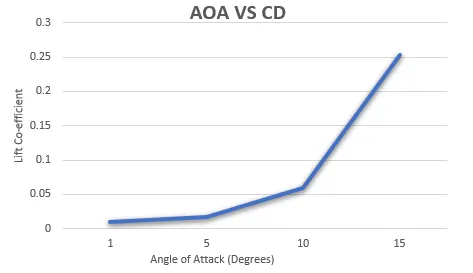
The above graph represents the plot of drag coefficient calculated at different angles of attack. As the angle of attack increases in AOA the value of drag coefficient increases smoothly up to a certain point and once the stalling angle is met the drag coefficient increases drastically, as the drag produced is greater during stalling when compared to the angle of attack of other values.

Angle of Attack vs Co-efficient of Lift:

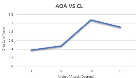
The above graph represents the plot of lift co-efficient calculated at different angles of attack. As the angle of attack increases we could observe an increases in lift co-efficient but after certain increase in angle of attack degree a stalling phenomenon occurs. A stall occurs when the angle of attack of an aerofoil exceeds the value which creates maximum lift as a consequence of airflow across it. This angle varies very little in response to the cross section of the airfoil.

Case 5:

Solver: K omega SST

Angle of Attack = 10 degree

Geometry:

Mesh:

Velocity Contour:

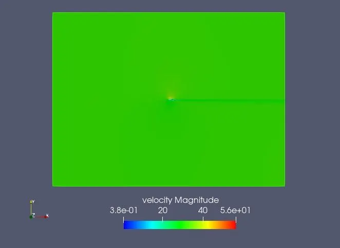
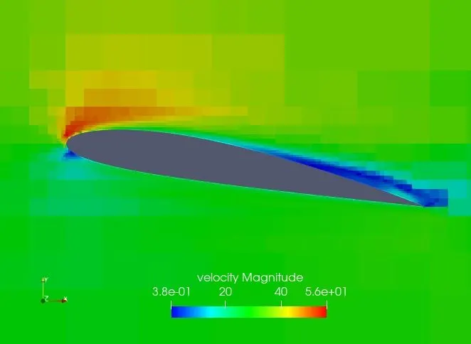
From the above contour plot we could observe that the velocity is clearly high on the upper surface of the airfoil and the velocity is lesser on the lower side of the airfoil. This is because of the airfoil geometry where the upper surface have a negative slope (curved downwards) where the air-molecules can move down easily and they also have their internal kinetic energy which increasess the velocity.

Pressure Contour:

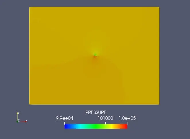
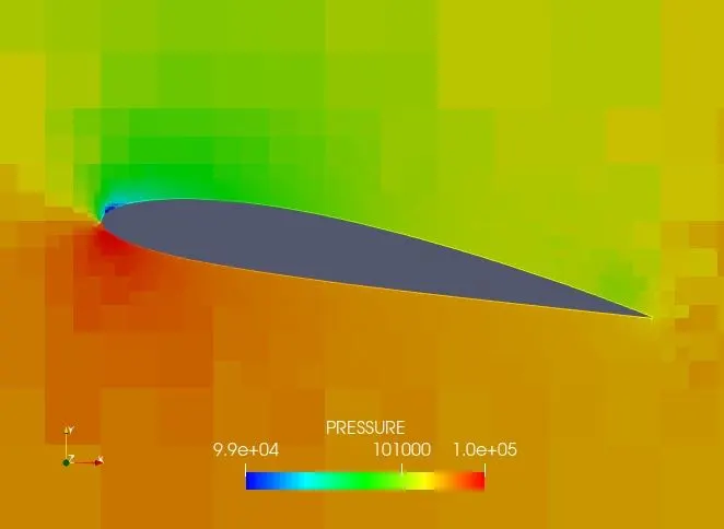
From the above contour plots we could predict that a low pressure region is created on the top of the airfoil because of its shape and velocity of the fluid.

Outlet Velocity:

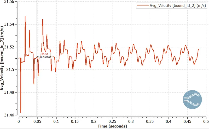
Pressure_Force_X (N):

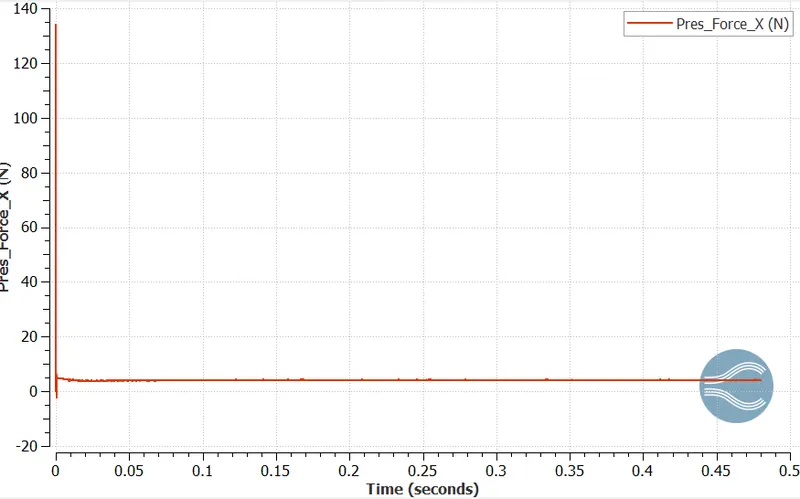
The above graph represents the pressure force in x-direction which is nothing but the drag produced by the airfoil body at a free stream velocity of 31.51 m/s

Pressure_Force_Y (N):

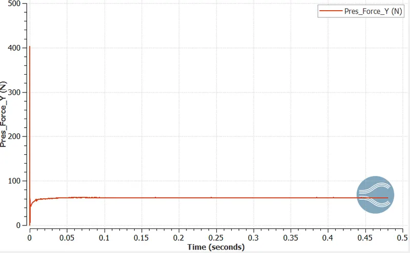
The above graph represents the pressure force in y-direction which is nothing but the lift produced by the airfoil body at a free stream velocity of 31.51 m/s

Hence from the above plots we could attain the value of drag and lift forces which can be used for calculating the co-efficient of drag and lift.

`F_D=4.10193`

`F_L=61.5482`

`rho=1.1765(kg)/m^3`

`A=0.1`

`v=31.51 m/s`

Drag Calculation:

`C_D=(2*F_D)/(rho*v^2* A)`

`C_D = (2*4.10193)/(1.1765*31.51^2*0.1)`

`therefore C_D=0.07023`

Lift Calculation:

`C_L=(2*F_L)/(rho*v^2* A)`

`C_L = (2*61.5482)/(1.1765*31.51^2*0.1)`

`therefore C_L=1.05379`

Co-efficient of Lift and Drag values for the airfoil at an angle of 10 degrees using RNG k-epsilon model is 0.0589 and 1.075 respectively.

Co-efficient of Lift and Drag values for the airfoil at an angle of 10 degrees using K omega SST model is 0.07023 and 1.05379 respectively.

K omega SST model was used for the angle of attack of 10 degrees to compare the results between the solver. From the results we could observe that the values for the drag and lift co-efficient differs. By observing the y plus value from k-epsilon turbulence model the values are in the log law region. In order to capture the effects more precisely we need to be in viscous sublayer which has low y plus. Hence, we can stick with k-omega turbulence model for better results.

Conclusion:

1. The flow over NACA 2412 airfoil at different angles of attack was simulated.
2. Transient state solver was used for overall simulation of this project.
3. The contours for velocity and pressure fields are plotted in order to study the behaviour of the fluid over the airfoil at different angles of attack.
4. Drag co-efficient and lift co-efficient plots were plotted against different angles of attack. Usage of two different turbulence models was carried out and their effects on simulation was studied.
5. The values in both turbulence model differs from each other. In order to capture the effects more precisely we need to be in viscous sublayer which has low y plus. Hence, we can stick with k-omega turbulence model for better results. K-omega SST turbulence model is well known for its uses in viscous sub layer.
6. Drag increases as the frontal area increases and also the lift increases until the flow undergoes flow separation.
7. It can be observed from the plot that the co-efficient of lift increases and co-efficient of drag increases at an angle of attack of 10 degrees, after that the co-efficient of lift decreases but the co-efficient of drag kept increases. This phenomenon is called stalling. This happens because of flow separation and formation of wide wake region over the surface of the airfoil.