Mini project - Flow over an Airfoil

AIM:

The aim of this project is to simulate the flow over a NACA 2412 aerofoil.

OBJECTIVES OF THE PROJECT:

• Simulate the flow for the following angle of attacks, Angle of attack = 1º, 5º, 10º,15º
• Find out the effect of drag coefficient Vs Angle of Attack
• Find out the effect of Lift coefficient Vs Angle of Attack
• Compare the effect of turbulence models on the above two parameters

THEORY:

What is an Aerofoil?

Aerofoil is the cross-sectional shape of a wing or a propeller blade. It is usually shown in the following figure.

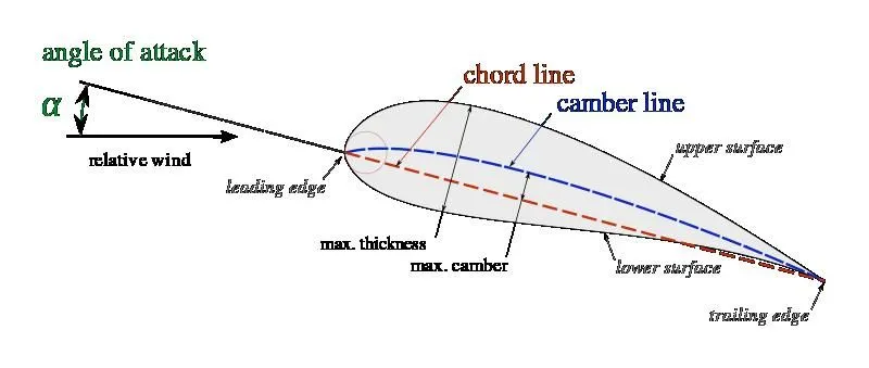
When air passes on any object it produces some lift and drag. Aerofoil is a shape optimized to produce more lift compared to drag. Aerofoil is not a fixed shape. But the usual idea is that on an aerofoil, air passing on the top should be faster than the air passing below the aerofoil. While satisfying the above condition we can create different aerofoils by altering the camber length and thickness.

In this project, my interest is to simulate airflow over NACA 2412 aerofoil. This aerofoil can be found at http://airfoiltools.com/. It is a huge library of different aerofoil shapes and their parameters.

PROCEDURE:

Creating the geometry

We start with creating geometry in SolidWorks. From the site, we take the formation in a DAT file and save it on our local computer. Then we copy the same data into an excel file and assign data according to spaces. The 2 columns indicate the coordinates on x and y. We add a third column which is all zeros, this is the z coordinates.

In Solid works,> Insert on the top panel > Curves > Curve through XYZ points > Here we paste the data we created in the excel file.

A curve will be created which we trace using the convert in the part sketch and extrude it to a certain length.

We save this part as an STL file from the save as options.

SETTING UP THE CASE

As we open a new project, we import the geometry by dragging it from the file explorer and dropping it on the converge screen or by importing it from the file menu.

Once the geometry appears, we need to check the geometry units. We can do this by going to the Left-side geometry panel > Options > check the boundary box.

If the boundary size is in the range of 100meters we can scale it by geometry panel > Transform > Scale > give a scaling factor of 0.001. And the geometry will come to a range of 0.1 m

The scale can be identified by calculating the speed required. For a Reynolds number of 200000, the velocity is

Re = (Rho of air * Velocity of air * Chord Length of aerofoil)/Dynamic viscosity of air

If the chord length is 1m then we get the velocity of the air as 3.12 m/s which is low to observe the effects of turbulence hence we take a chord length of 0.1m and we get the velocity of air as 31.2 m/s.

Here we can observe the airflow using a wind tunnel. We carve a hole in the shape of this aerofoil in a rectangular box and give airflow in that rectangle. And we can observe the airflow from the side of that rectangle.

To create the wind tunnel, we create a box using the create option and input the dimensions as 1.25 for x and 0.75 for y, and 0.02 for z

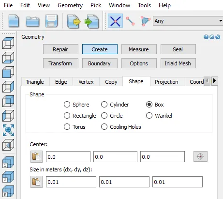
The wind tunnel dimensions are usually 50 times the chord length in the x-direction, 30 times the chord length in the y-direction. But the cells required to perform calculations are too large and the simulation would be very time-consuming. So, we reduce the wind tunnel size.

Now we delete the side faces of the wind tunnel and patch them with the vertices on the aerofoil using patch using ordered vertex list. This will create a hole in the wind tunnel.

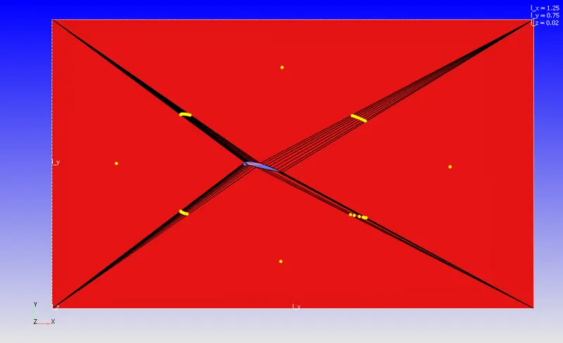
In the “Boundary” options select flag and press “+” select 6 boundaries and press ok. We keep the geometry in standard orientation.

6 boundaries will be shown, we rename them as

Boundary 1 > “Airfoil” (Select all the triangles on the airfoil.)

Boundary 2 > “Inlet” (select all the triangles on the left.)

Boundary 3 > “Outlet” (Select all the triangles on the right.)

Boundary 4 > “Top and bottom” (select all the triangles on the top and bottom.)

Boundary 5 > “Front 2D” (Select all the triangles on the front.)

Boundary 6 > “Back 2D” (Select all the triangles at the back.)

• Now left-click on a boundary name and select the triangles on the geometry to assign those triangles to the boundary. Repeat this process for both the boundaries created.
• We can make sure that all the boundaries are assigned by checking the Not Assigned (Boundary ID 0), If the triangles in this boundary are none then all the triangles are assigned to the created boundaries.

The normal in geometry should point towards the fluid domain. Invert the normal towards the inside where the fluid is flowing.

We first set up a steady-state case

In the run parameters in the solver: select the steady-state solver, make sure the simulation mode is set to full hydrodynamic Gas flow solver: Compressible.

• In the miscellaneous tab uncheck the use shared memory option and click on ok.

The type of solver will be set to transient in the transient condition and a steady-state monitor is not necessary for the transient case.

This selects the type of solver to be used for our case.

• In the Simulation, time parameters enter the following values.

Start time: 0 cyc

End time: 20000 cyc

Initial time step: 1e-9s

Minimum time step: 1e-9s

Maximum time step: 1s

Maximum convective CFL: 0.8 click on ok.

• In the solver parameters section select the Density-based option.

In the steady-state monitor, we configure the total pressure and average velocity and proceed to boundaries and regions.

Now before we go into the boundaries option click on regions and initialization. Click on add new region. Right-click on region 0 and rename it to high pressure. On the left side near the species click on + and add air and select the temperature as 300k and pressure as 101325pa and velocity to 31.2m/s.

The airfoil, Top, and bottom are walls with slip condition for top and bottom and law of wall condition for Airfoil. and assign the region for all the boundaries.

And make sure the inlet boundary velocity is a specified value of 31.2m/s.

• In the physical models > Turbulence modeling select the RANS option and select Komega SST and press ok.
• In the Grid control select the Adaptive mesh refinement option and press ok. A new option appears in grid control called “Adaptive mesh refinement”
• In the Grid Control > Base Grid > set the x, y, z sizes to 2.5e-4m and click ok.
• In the Adaptive mesh refining option. Select the minimum number of cells to 1 and the maximum number of cells to 3,00,000. And add the High pressure and low-pressure regions to active regions. In the bottom Velocity tab select the Default embedding level: 4
• Select the type: sequential and select the SGS embed to 0.1; and start and end time for amr as 0 and 20000 cyc

We then set the output file settings and export the files and run the simulation

Upon running the steady-state simulation, we get the following results.

Steady State K omega SST

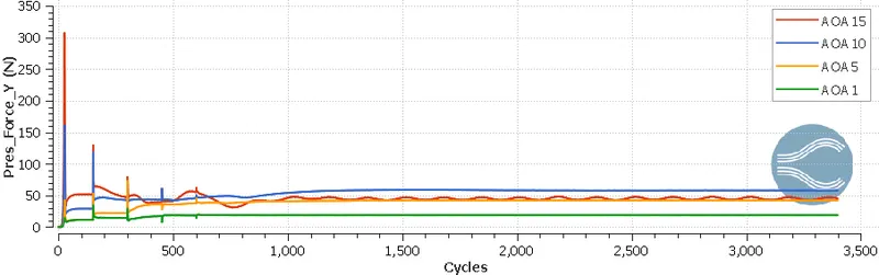
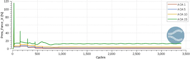
The above plots indicate the lift and drag produced in different angles of attacks for a steady-state simulation. And we can see that as the angle of attack reached 15 degrees the oscillations in the solution increased. To achieve a more stable solution a transient case is tested.

The flow-through time is found to be 1.6sec we can round it off to the next value, So the time duration is 2 secs and all the other parameters remained the same. And the following graphs are obtained.

Transient k omega SST

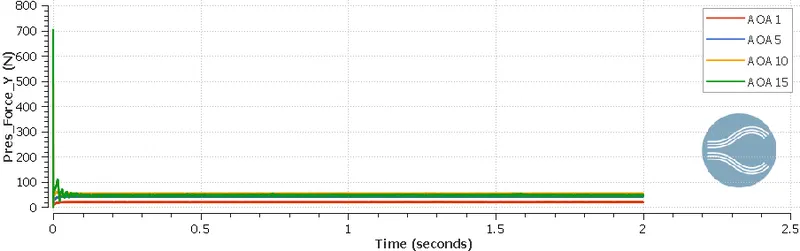
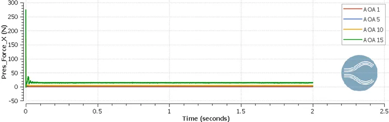
We can see that for a transient case the oscillations reduced, and we are at a much more stable solution.

From the pressure obtained, the coefficients of drag and lift are calculated and are plotted using octave. This program required io package to be loaded into OCTAVE

Upon running the above program, we get the following plots

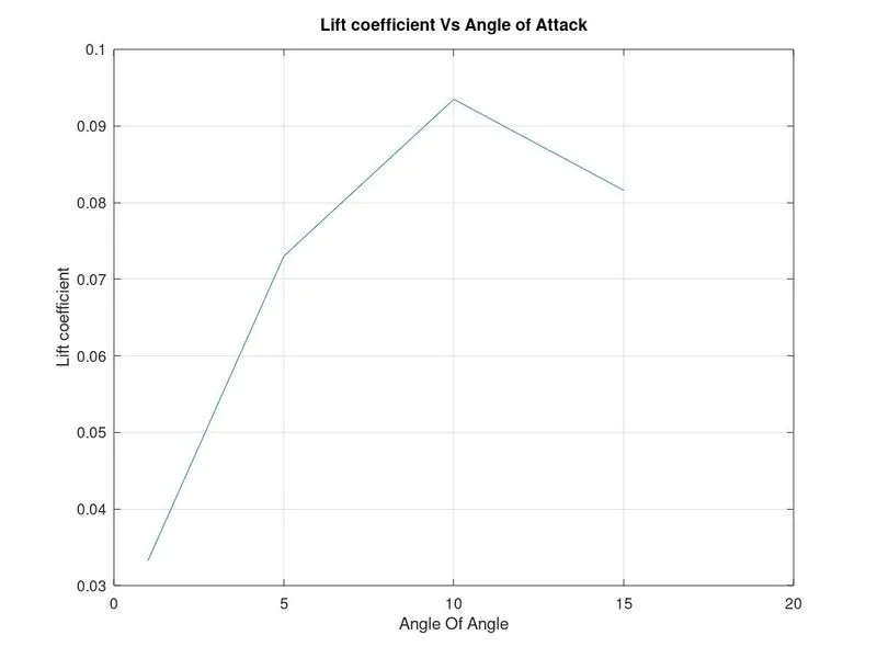
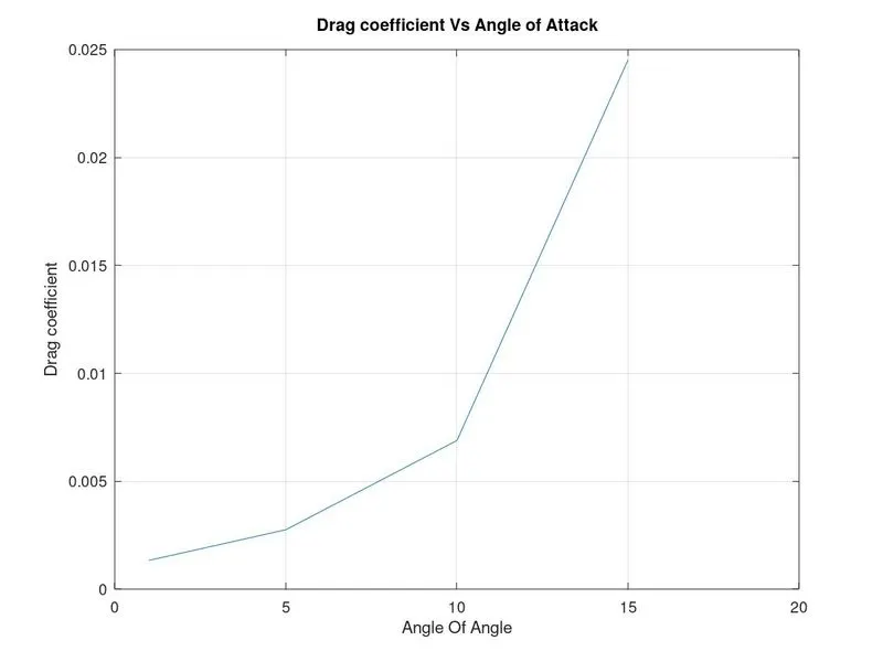
The above plots are meaningful as they show how the lift coefficient changes with the angle of attack and it is what would happen in a real flight.

To check the effect of the turbulence model, the above simulation is made to run with a different turbulent model which is RNG k-epsilon, and the following results are obtained.

RNG k epsilon

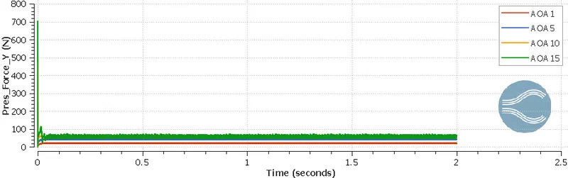
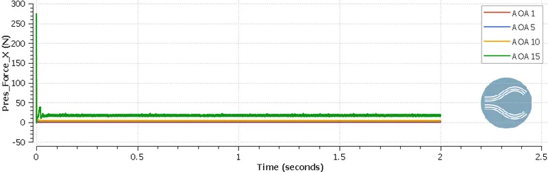
We can see that the solution deviation is more. This could possibly be caused due to the change in y plus. The RNG k epsilon method is suitable for yplus values above 30 and the k omega SST is suitable for a low y plus value <10. Due to this the accuracy at the wall decreases as the cell height is wrongly estimated and this leads to a less accurate value in the solution.

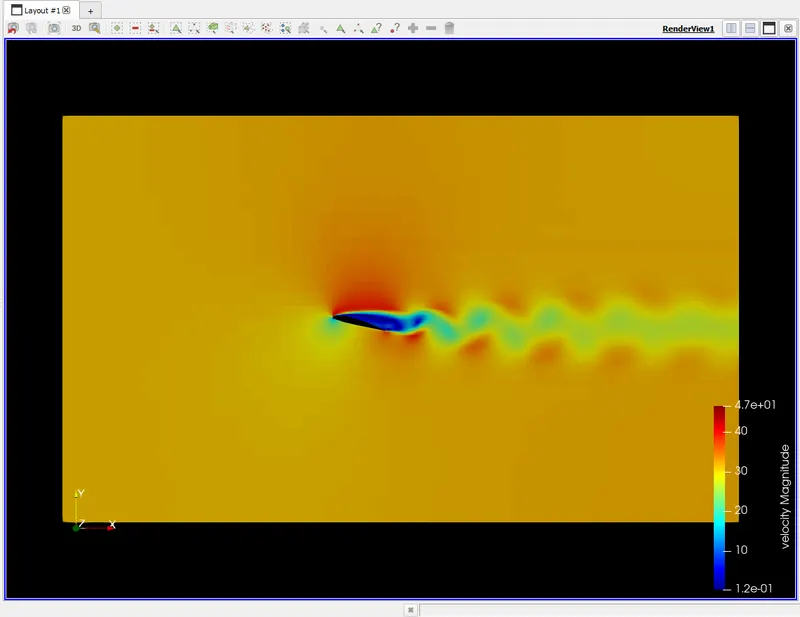
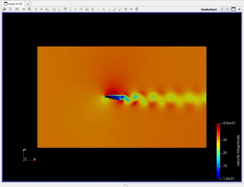
The velocity contours for the above three methods look similar but there are some differences as well

Steady State

Transient with K omega SST

Transient with RNG K epsilon

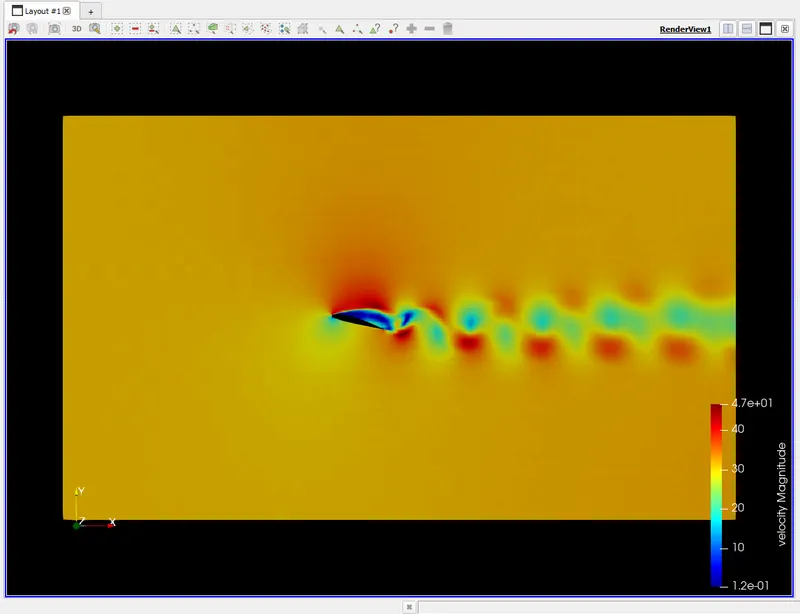
The above graphs are generated for a 15 degree Angle of Attack. In a real-world test for a 15-degree angle of attack, the lift would decrease and the turbulence increases because of vortex shedding. It can be observed that the vortices are much more clearly visible in transient cases than the ones in a steady state. Also If we compare the effects at the aerofoil, In the RNG K epsilon the velocity profile at the aerofoil indicates there is an increase in the velocity at the midpoint of the chord which is impractical unless there is a decrease in the area of the cross-section. We can see that the K omega SST model predicted this much more accurately.

Conclusion

From the above results, the following observations are made

• The converge's steady-state solver is not suitable for this simulation.
• The transient case is much more effective and the K omega SST model calculates the physics better than RNG K epsilon.