Matlab program to plot Pressure-volume graph of an Otto cycle

AIM: The aim is to write a program in MATLAB that can solve an Otto cycle and plots for it.

OBJECTIVES:

The code should create a PV diagram representing the pressure and volume at various stages of a PV diagram

Also, the thermal efficiency of the engine is to be calculated.

GOVERNING EQUATION:

The above equation is derived from geometrical relationships in an IC engine arrangement. For more clarification regarding this equation refer to the following link

https://www.engr.colostate.edu/~allan/thermo/page2/page2.html#:~:text=The%20volume%20of%20the%20piston,bore%20and%20connecting%20rod%20length.&text=The%20final%20form%20of%20the,(6)%20by%20Vd.

The units considered for

Pressure = pascal

Volume = m^cube

Bore, stroke, connecting rod length = m

Temperature = kelvin

Theta is taken in degrees (sind and cosd commands are used)

BODY OF THE CONTENT:

This program assumes that the gas used in the process is an ideal gas

A MATLAB program is written to find the pressure and volume at various stages of the cycle using the general gas equation and the isentropic pressure-volume relation.

1. To start with the program inputs bore diameter, stroke length, connecting rod length, compression ratio, t1, p1, t3, gamma is taken.
2. We know that

Vswept = (∏/4) *((bore_dia) ^2) *stroke

3. Also

Clearance = Vswept/(cr-1) (cr is the compression ratio)

4. Adding the equations in points 2 and 3

we get v1 = Vswept + clearance

5. Since v1/v2 = cr we can find out the v2
6. Using the isentropic equation

p1*(v1^gamma) = p2*(v2^gamma)

7. We can find out the value of p2
8. Now using the general gas equation, we can also find out the temperature at the second stage using the formula

p1v1/t1 = p2v2/t2

9. Now we have p2, v2, t2 we know that the process from stage 2 to stage 3 is a constant volume adiabatic heat addition

v2 = v3

10. Since we know the t3, v3 we can find out the p3 using general gas equation i.e.,

P2v2/t2 = p3v3/t3

11. So now the p3, v3, t3 are found out we can find the pressure, volume, the temperature at the fourth stage

We know that at the fourth stage the volume is the same as stage one

Hence v4 = v1

12. Using the isentropic equation, we get p3*(v3^gamma) = p4*(v4^gamma) we can find the value of p4
13. Again, using the general gas equation, we can calculate the value of t4 using

P3v3/t3 = p4v4/t4

14. We have the points we can use to plot the graph but we don’t know how the volume changes i.e., the volume change won’t be a straight line so we need to find out the path taken by the volume
15. So to solve this problem if we can find out how the volume changes with respect to the angle made by the crank we can use that information to plot the graph
16. Picture credits to skill Lync
17. The above equation is used for finding out the volume change with respect to crank angle in the above equation vc is the clearance volume, rc is the compression ratio,

Connecting rod length

R = -------------------------------- ; where a = strokelength*0.5 ; Ɵ is the crank angle

a

18. By plugging in the known values in the above equation we can get the values of V
19. We use a linspace command for theta we can have a range of V
20. After getting the required values we create a function named piston_kinematics
21. We can call this function in our main program so that we can get a range of values for Vcompression and Vexpansion when required

(Note: the function piston_kinematics needs to be stored in the same directory where our main program is stored else the function won’t work)

22. So now we call this function near 1-2 and 3-4 by using the values of 180 to 0 and 0 to 180 at compression and expansion respectively to get the values of Vcompression and V expansion
23. Using the relation p1*(v1^6gamma) = constant1; p3*(v3^gamma) = constant = c2

And P compression. *(Vcompression. ^gamma) = constant1

P expansion. *(V expansion. ^gamma) = constant2

24. Now we can use the plot command to plot all the required graphs.
25. For finding out the thermal efficiency of the cycle we know that the

Thermal efficiency = work done/heat supplied

Work done = q23 + q41 and heat supplied = q23

So therefore, thermal efficiency = (q23 + q41)/q23

= 1 + (q41/q23)

= 1 - (-q41/q23)

= 1 – {[Cv(t4-t1)]/[Cv(t3-t2)]}

= 1 – [t4-t1]/[t3-t2]

26. Plugin the values of known T’s and we get the thermal efficiency

RESULTS:

The value of thermal efficiency obtained with the values taken from the program is 62.9892%

(The stepwise explanation of the program written is explained in the program pasted below)

(The main program)

 clear all
 close all
 clc
 
 %state variables
 gamma  = 1.4;
 %pressure(pa = N/m^2)
 P1 = 101325;
 %Temperature(kelvin)
 T1 = 500;
 T3 = 2300;%assuming t3 is given
 
 %to calculate V1 lets use engine parameters and these parameters also help
 %us in finding the volume track i.e which path V1 takes to V2(m)
 bore = 0.1;
 stroke = 0.1;
 conrod_length = 0.15;
 %compression_ratio
 cr =  12;
 
 %calculating the swept volume and the clearance volume
 V_swept = (pi/4)*bore^2 *stroke;
 V_clearance = V_swept/(cr-1);
 
 V1 = V_swept + V_clearance
 V2 = V1/cr
 
 %calculating state variables at 2nd state
 %WKT for an isentropic process p1*v1^gamma = p2*v2^gamma
 %P2 = P1(V1/V2)^gamma i.e  P2 = P1*(cr)^gamma
 P2 = P1*(cr)^gamma
 
 
 %from piston kinematics we got the vcompression
 
 V_compression = piston_kinematics(bore,stroke,conrod_length,cr,180,0)
 %during the compression the crank goes from 180 to 0 and during the
 %expansion the crank goes 0 to 180
 
 %WKT in an isentropic process pv^gamma = constant
 %so if we know the constant we can find out Pcompression
 %finding out the constant
 
 constant_c = P1*(V1^gamma);
 
 %now using P_compression = constant(c)/(V_compression^gamma)
 
 P_compression = constant_c./(V_compression.^gamma);
 
  
 %using the formula p1v1/t1 = p2v2/t2
 T2 = P2*V2*T1/(P1*V1)
 
 %calculating state variables at state 3
 %WKT 2-3 is a constant volume process hence v2= v3
 V3 = V2;
 
 %again using the formula p2v2/t2 = p3v3/t3
 P3 = P2*T3/T2
 
 
 %calculating the state variables at state 4
 %WKT the volume at the end of the process is the same as the volume at state 1
 V4 = V1 
 
 %pressure can be found by using the p1v1^gamma = p2v2^gamma
 %p2 =  p1(v1/v2)^gamma
 P4 = P3*(V3/V4)^gamma
 
 %using the general gas equation we get the value of t4
 T4 = P4*V4*T3/(P3*V3)
 
 %Using the similar logic we used for compression
 V_expansion = piston_kinematics(bore,stroke,conrod_length,cr,180,360);
 
 constant_c1 = P3*(V3^gamma);
 P_expansion = constant_c1./(V_expansion.^gamma);
 
 
 %plotting
 figure(1)
 hold on
 plot(V1,P1,'*','color','b')
 plot(V2,P2,'*','color','b')
 plot(V_compression, P_compression)
 plot(V3,P3,'*','color','b')
 plot([V2 V3],[P2 P3])
 plot(V4,P4,'*','color','r')
 plot(V_expansion, P_expansion)
 plot([V4 V1],[P4 P1])
 xlabel('volume')
 ylabel('pressure')
 %to know the exact path in which v1 goes to v2 i.e is how the volume
 %changes in the combustion chamber we need to know how the piston moves to
 %take a reference we find out how the piston moves with repsect to crank
 %angle piston_kinematics.m
 
 
 %thermal efficiency of this cycle is calculated using
 tempdiff_top = T4 - T1;
 tempdiff_bottom = T3 - T2;
 tempdiff_divided = tempdiff_top/tempdiff_bottom;
 thermal_efficiency = (1 - tempdiff_divided)*100;%in percentage
 

(The function part)

%This program is to find out the piston kinematics which will help us
%understand how the piston moves with respect to the crank angle in the
%combustion chamber. We create a function in this program and we use this
%function in the ottocycle_example.m program

function [V] = piston_kinematics(bore, stroke, conrod_length,cr,start_crank,end_crank)
%so the function gives an ouput called V and it requires the variables in
%the brackets shown following the same order

%getting the same engine parameters from ottocycle_example.m
a = stroke/2 %crank pin radius
R = conrod_length/a %ratio of connecting rod length to crank pin radius


%computing swept volume and clearance volume
V_swept = (pi/4)*bore^2*stroke
V_clearance = V_swept/(cr-1)
V1 = V_clearance + V_swept;

theta = linspace(start_crank,end_crank,100); %the angle made by the crank with reference axis the piston axis

%since the governing equation is big we divided it into 3 terms
term1 = 0.5*(cr-1);
term2 = R+1-cosd(theta);
term3 = [(R^2)- sind(theta).^2].^0.5;

V = [1+term1*(term2-term3)]*V_clearance;
%plot(theta,V,''linewidth',3)
end

OUTPUT PLOT:

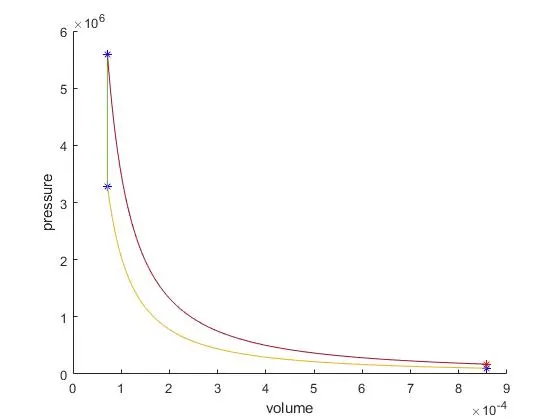
CONCLUSION:

A graph representing the pressure and volume at various stages and how the pressure and volume change stage in an Otto cycle has been plotted. The same procedure can be used to plot graphs for any other air standard cycle. However, this project has been made lengthy for a better understanding of formulas in order to reduce the length of the code general gas equations and isentropic gas equations can be made as functions and can be called whenever required.