Rankine cycle simulation using Matlab

AIM:

The aim of this project is to write a MATLAB code to simulate the Rankine cycle.

OBJECTIVES OF THE PROJECT:

The main objectives of this project are

• To calculate the state point variables of the Rankine cycle based on user inputs.
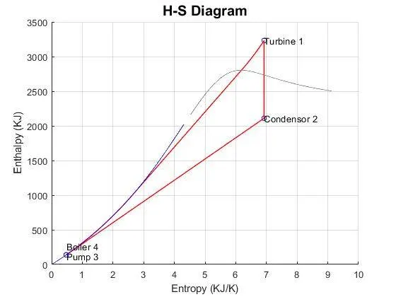
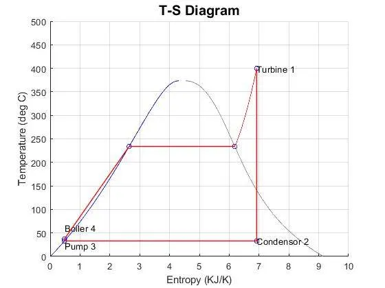
• To plot the H-S, T-S diagrams for the given inputs.
• To calculate the Net-work output and the back-work ratio.

BODY OF THE CONTENT:

Before writing a MATLAB program, A quick glance at the Rankine cycle would brush up the basics.

RANKINE CYCLE is also known as a modified Carnot cycle. It is used to predict the performance of reciprocating steam turbine systems. It is an idealized thermodynamic cycle of a heat engine that converts heat into mechanical work while undergoing a phase change. The following picture shows the different stages of a Rankine cycle.

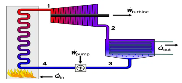
Picture credits skill lync

Power generation is dependent on the temperature depending on the temperature difference between a heat source and a cold source. This can also be used in powerplants.

The cycle usually starts from the boiler. But for our convenience here we took the turbine as stage1. The process from

1-2 ISENTROPIC EXPANSION

Steam is expanded in the turbine in an isentropic process hence the entropy change in this process would be zero. While the steam expands it rotates the turbine producing some work. This work can be denoted by using

since ∆Q = 0; work produced in the turbine is W turbine = h1-h2

2-3 CONSTANT PRESSURE HEAT REJECTION

Steam expanded in the turbine has some temperature this is made to lose using the heat exchangers in the condenser. So as the steam losses heat it undergoes a phase change and is converted into water. This process happens while keeping the pressure constant.

∆P = 0 this implies that W = 0

Therefore Q = h2 – h3

3-4 ISENTROPIC COMPRESSION

The steam-water mixture now needs to be again pumped back into the boiler, so a pump is used to pump the steam-water mixture back into the boiler. During this, the steam is compressed in an isentropic process.

since ∆Q = 0; work done by the pump is W pump = h4-h3

4-1 CONSTANT PRESSURE HEAT ADDITION

The steam-water mixture is pumped into the boiler where heat is added to the water mixture to convert the entire water into steam that can be utilized to produced useful work.

Again, ∆P = 0 this implies that W = 0

Therefore Q = h1– h4

Net-work produced in the cycle is given by removing the word used by the pump from the work produced in the turbine.

Wnet = Wturbine – Wpump

Wnet = h1- h2-h4+h3 KJ/kg

Steam rate is given as 3600/Went Kg/KWh

The back work ratio is given by the Back work Ratio: Wpump/Wturbine.

The given inputs are

Turbine inlet temperature: 400 °C

Turbine inlet pressure: 30 bar

Turbine exit pressure = Condenser inlet pressure : 0.05 bar

In order to solve the Rankine cycle, we need steam values. We use the XSteam library for obtaining the values

Starting from state 1

We know that P1 = 30 bar and p2 = 0.05 bar since two processes in 4 are at constant pressure we have p3 = p2 and p4 = p1

We have temperature given 400 °C at pressure 30 bar we use the XSteam library to get the saturation temperature of steam at 30 bar if the given temperature of steam at 30 bar is greater than the saturated temperature then the steam is at a superheated state.

Now for the temperature and pressure using the Xsteam library, we obtain the enthalpy at state 1

For enthalpy at state 2

We know that the process 1-2 is isentropic hence S1 = S2. We obtain S1 by using the temperature and pressure at state 1

S2 = Sf2 – X* Sfg2

We know the values of S2, we use the xsteam to values sf2 and sg2

sfg2 = sg2 – sf2. Plugging in all the values we get the value of dryness fraction X

Now we use h2 = hf2 – X*hfg2

We use the xsteam to find out the hf2 and hfg2, Also the hf2 is nothing but h3

In order to find h4 we need to use another method

We know that work done by pump is nothing w = h4 – h3

Also, w = vdp = v3 (p4 – p3) so v3 can be obtained by using the xsteam library

So now we can get h4 as for the entropies s1 = s2 and s3 = s4 so if we can look those values up in XSteam as well

To find out the temperatures we know that the temperature drops during the expansion in the turbine hence the dropped temperature can be looked up in the steam library at p2 and h2 so the t3 will be equal to t2 since the temperature drops between the processes are assumed to be neglected.

Now in the boiler water is heated and the temperature rises to t4 this can be calculated using the cp, cv relations.

Cp, Cv at p4 h4 are obtained using the steam table

Now k = Cp/Cv we know that the temperature change relation is obtained using

T1/T2 = (P1/P2) ^((k-1)/k)

we use the above relation for obtaining the t4 using the t3

Now the entropies at saturated points s5 liquid state and s6 gas state are obtained by using the pressure in the XSteam library.

Now we have everything required we plot the HS and TS diagrams.

MATLAB PROGRAM

clear all        
close all 
clc

%This Program finds out the Network done, Backwork ratio in a Rankine cycle 

fprintf('ntttttttt Rankine Cycle Simulatornnn')

%Inputs
%For easy understanding i chose the turbine phase as 1st step
fprintf('ttprocess:1-2 indicates isentropic expansion in the turbinen');
fprintf('ttprocess:2-3 indicates Constant pressure heat rejection in the turbinen');
fprintf('ttprocess:3-4 indicates isentropic expansion in the Pumpn');
fprintf('ttprocess:4-1 indicates Constant pressure Heat addition in the boilernn');

%Turbine Inlet Temperature  
T(1) = input('        What is the Temperature at the Turbine inlet(in Degree Celcius)');

%Turbine inlet pressure (Bars)
P(1) = input('        what is the pressure at turbine inlet(in bar)') ;

%Turbine Outlet pressure (Bars)
P(2) = input('        What is the pressure at turbine exit (in bar)') ;

%The exit pressure of the turbine is the same as the inlet pressure of the
%condensor therefore
P(3) = P(2);

%As the water passes through the pump the inlet pressure will be the same as
%the exit pressure of the condenser and the inlet pressure of the boiler
%will be the same as the inlet pressure of the turbine therefore
P(4) = P(1);

%We start with finding out the enthapy at all the points starting with
%turbine end
h(1) = XSteam('h_pT',30,400);

%Now that we got the enthalpy at the turbine lets find out the enthalpy at
%the condenser
%To find out the value of the enthalpy we know that the expansion in the 
%Turbine is isentropic therefore the entropy S1 and entropy S2 that is
%after the condenser is the same Hence

S(1) = XSteam('s_pT',30,400);

S(2) = S(1);

%Also we know that entropy before the turbine phase can be broken down into
% S1 = Sf + (X).(Sfg)
%The above equation is manipulated to find out the X i.e., Dryness
%Fraction.

Sf1 = XSteam('sL_p',0.05);
Sg1 = XSteam('sV_p',0.05);
Sfg1 = Sg1 - Sf1;

X  = (S(1) - Sf1)/Sfg1 ;

S(3) = XSteam('sL_p',0.05) ;

S(4) = S(3);

S(5) = XSteam('sL_p',P(1));

S(6) = XSteam('sV_p',P(1));

% By Using this dryness fraction we find out the Enthalpy at the 2nd point
% using 

hf1 = XSteam('hL_p',0.05);
hg1 = XSteam('hV_p',0.05);
hfg1 = hg1 - hf1;

h(2) = hf1 + (X*hfg1);

h(3) = hf1 ;

%For finding the h4 We use a different approach
%We know that Work Done by the Pump WD = h4 - h3
%But Work is done by the pump can also V3(P4-P3)
% point 3 is exactly at the liquid phase of the dome of the TS diagram
%hence V3 is nothing but specific volume Vf.

V3 = XSteam('vL_p',0.75);

Wpump = abs(V3*(P(4)-P(3))*100);

h(4)  =  Wpump + h(3);

%Now we have enthalpies at each and every stage we can find out

%%%%%%%%%%%%%%%%TEMPERATURES%%%%%%%%%%%%%%%%%%%%%%%%%%%%%%
% Temperature at a stage can be found out using the XSteam
T_sat = XSteam('Tsat_p',P(1),h(1));

T(2) = XSteam('Tsat_p',P(2));
T(3) = T(2);
cp4 = XSteam('Cp_ps',P(4),S(4));
cv4 = XSteam('Cv_ps',P(4),S(4));
k = cp4/cv4;
kterm = (k-1)/k;
invterm = (P(4)/P(3))^kterm;
T(4) = T(3)*invterm ;
T(5) = T_sat;

% NET work  = WORKturbine - WORKpump

Wtur =  (h(1)-h(2));

Wnet = (Wtur - Wpump);

%Also the back work ratio is the ratio of work done by the pump to the work done
%by the Turbine

Bwr = Wpump/Wtur;

S_S_C = 3600/(Wnet);

Qin =  (h(1)-h(4));

eff = ((Wnet/Qin))*100;

%fprintf('%35sn','RESULTS')

fprintf('ttThe saturation temperature of steam at state 1 i.e %f bar  has been checkedn',P(1))
fprintf('ttAnd is found to be %f and the given input temp is %fn',T_sat,T(1));
fprintf('ttSince the state1 temperature is higher than the saturation temperature the steam is at super heated statenn')

%Results 
fprintf('ntttttttt RESULTS  nn')
fprintf('tt At statepoint : 1 tttttt')
fprintf('At state point : 3 n')
fprintf('tt T1 = %f Degrees celciustt',T(1))
fprintf('T3 = %f Degrees celciusn',T(3))
fprintf('tt P1 = %f bartttttt',P(1))
fprintf('p3 = %f barn',P(3))
fprintf('tt h1 = %f KJ/Kg tttt',h(1))
fprintf('h3 = %f KJ/kgn',h(3))
fprintf('tt s1 = %f KJ/KgK ttttt',S(1))
fprintf('s3 = %f KJ/kgKn',S(3))
fprintf('tttttttttttt')
fprintf('n')

fprintf('tt At statepoint : 2 tttttt')
fprintf('At state point : 4 n')
fprintf('tt T2 = %f Degrees celciusttt',T(2))
fprintf('T4 = %f Degrees celciusn',T(4))
fprintf('tt P2 = %f bartttttt',P(2))
fprintf('p4 = %f barn',P(4))
fprintf('tt h2 = %f KJ/Kg tttt',h(2))
fprintf('h4 = %f KJ/kgn',h(4))
fprintf('tt s2 = %f KJ/KgK ttttt',S(2))
fprintf('s4 = %f KJ/kgKn',S(4))
fprintf('tttttttttttt')
fprintf('n')

fprintf('tt Pump work %fn',Wpump);
fprintf('tt Turbine work %fn',Wtur);
fprintf('tt Net work %fn',Wnet);
fprintf('tt Efficiency %fn',eff);
fprintf('tt Specific Steam Consumption %fn',S_S_C);
fprintf('tt BackWork Ratio %fn',Bwr);


%For the construction water saturated and superheated value dome
%We take some temperature range and for each temperature we find out the
%entropies and enthalpies at gaseous and liquid states we get the dome
t= linspace(0,500,500);
for i = 1: length(t)
    wSL(i)   = XSteam('sL_T',t(i));
    wSV(i)   = XSteam('sV_T',t(i));
    wHL(i)   = XSteam('hL_T',t(i));
    wHV(i)   = XSteam('hV_T',t(i));
end

%Plotting HS diagram
figure(1)
hold on
grid on
plot(S(1),h(1),'o','markersize',5,'color','b')
text(S(1),h(1),'Turbine 1')
plot(S(2),h(2),'o','markersize',5,'color','b')
text(S(2),h(2),'Condensor 2')
plot(S(3),h(3),'o','markersize',5,'color','b')
text(S(3),h(3)-20,'Pump 3')
plot(S(4),h(4),'o','markersize',5,'color','b')
text(S(4),h(4)+120,'Boiler 4')
s23 = linspace(S(2),S(3),100);
s45 = linspace(S(4),S(5),100);
s56 = linspace(S(5),S(6),100);
s61 = linspace(S(6),S(1),100);
for r = 1:length(s45)
    h23(r) = XSteam('h_ps',P(1),s23(r));
    h45(r) = XSteam('h_ps',P(1),s45(r));
    h56(r) = XSteam('h_ps',P(1),s56(r));
    h61(r) = XSteam('h_ps',P(1),s61(r));
end
plot([S(1) S(2)],[h(1) h(2)],'linewidth',1,'color','r')
plot([S(3) S(4)],[h(3) h(4)],'linewidth',1,'color','r')
plot([S(2) S(3)],[h(2) h(3)],'linewidth',1,'color','r')
%plot([S(4) S(1)],[h(4) h(1)],'linewidth',1,'color','r')
plot(s23,h23,'linewidth',1,'color','r')
plot(s45,h45,'linewidth',1,'color','r')
plot(s56,h56,'linewidth',1,'color','r')
plot(s61,h61,'linewidth',1,'color','r')
plot(wSL,wHL,'linewidth',1,'color','b')
plot(wSV,wHV,'linewidth',1,'color',[0.5 0.5 0.5])
title('H-S Diagram','fontsize',15)
xlabel('Entropy (KJ/K)')
ylabel('Enthalpy (KJ)')

%Plotting TS diagram
figure(2)
hold on
grid on
plot(wSL,t,'linewidth',1,'color','b')
plot(wSV,t,'linewidth',1,'color',[0.5 0.5 0.5])
plot(S(1),T(1),'o','markersize',5,'color','b')
text(S(1),T(1),'Turbine 1')
plot(S(2),T(2),'o','markersize',5,'color','b')
text(S(2),T(2),'Condensor 2')
plot(S(3),T(3),'o','markersize',5,'color','b')
text(S(3),T(3)-10,'Pump 3')
plot(S(4),T(4),'o','markersize',5,'color','b')
text(S(4),T(4)+25,'Boiler 4')
plot(S(5),T(5),'o','markersize',5,'color','b')
plot(S(6),T_sat,'o','markersize',5,'color','b')
plot([S(1) S(2)],[T(1) T(2)],'linewidth',1,'color','r')
plot([S(3) S(4)],[T(3) T(4)],'linewidth',1,'color','r')
S45 = linspace(S(4),S(5),1000);
for j = 1: length(S45)
    T45(j) = XSteam('T_ps',P(1),S45(j));
end
plot([S(4) S(5)],[T(4) T(5)],'linewidth',1,'color','r')
S11 = linspace(S(6),S(1),1000);
for k = 1:length(S11)
    T11(k) = XSteam('T_ps',P(1),S11(k));
end
plot([S(2) S(3)],[T(2) T(3)],'linewidth',1,'color','r')
plot([S(5) S(6)],[T(5) T_sat],'linewidth',1,'color','r')
plot(S11,T11,'linewidth',1,'color','r')
axis([0 10 0 500])
title('T-S Diagram','Fontsize',15)
xlabel('Entropy (KJ/K)')    
ylabel('Temperature (deg C)')

OUTPUT WINDOW

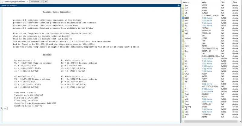
PLOTS

5.CONCLUSION:

• The efficiency of the Rankine cycle is found to be 36% approx. which can be improved further by using reheat or regenerative Rankine cycle. This project plots the approximate values of the state points without the XSteam library it will be difficult to plot the state points.

REFERENCES

Rankine cycle - Energy Education

How to solve Rankine cycle questions(solved example by using STEAM TABLE) - YouTube