Matlab program to solve ODEs
AIM: The aim of this challenge is to write a program in MATLAB that can solve an Ordinary differential equation plots the data and simulates it accordingly.
OBJECTIVES:
- To write a MATLAB program that can solve an ODE. The ODE is the equation of motion of a simple pendulum with damping.
- Simulate the motion between 0-20 sec, for angular displacement=0, angular velocity=3 rad/sec at time t=0.
GOVERNING EQUATION:
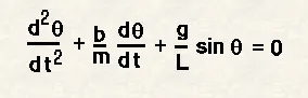
The way the pendulum moves depends on Newton's second law. When this law is written down, After doing some mathematical operations we get a second order Ordinary Differential Equation that describes the position of the ball w.r.t time as: -
(Picture credits to skill Lync)
In the above equation,
g = gravity in m/s2,
L = length of the pendulum in m,
m = mass of the ball in kg,
b=damping coefficient.
Theta is taken in degrees (sind and cosd commands are used)
PROCEDURE:
We use some inputs to solve the above equation such as
L=1 metre, m=1 kg, b=0.05. g=9.81 m/s^2, timespan = 20sec, defined using the linspace command.
INITIAL CONDITION: angular displacement = 0, angular velocity=3 rad/sec at time t=0,
A MATLAB program is written using the ode45 function to solve the given equation with the given inputs and the initial conditions.
Before stepping into the program, we need to arrange the method we use to solve the equation this includes the rearranging of the given ode. In what way we rearrange it depends on.
ODE45 is a function in MATLAB that can be used to solve Ordinary as well as partial differential equations. This uses a numerical method called the Runge Kutta method of 4th order. Normally for solving a differential equation we usually solve it by integrating it over a limit and we plug in the limit values to get a solution for the unknown. Instead of direct integration, we can discretize the equation i.e., we convert the given equation into a linear equation and solve it using the Runge Kutta method to get an approximate solution.
RUNGE KUTTA METHOD :
- It requires an initial condition y (0)
- Step size (h) or (time step)
For e.g. if there is a problem y’ = f(t,y) we need to find out four terms
K1 = f (Tn,Yn)
K2 = f (Tn + (h/2), Yn+((h/2). K1)))
K3 = f (Tn + (h/2), Yn+((h/2). K2)))
K4 = f (Tn + (h/2), Yn+((h/2). K3)))
Now,
Yn+1 = Yn + (K1/6) +(K2/3) +(K3/3) +(K4/6),
The above equation gives an approximated value of the solution of Y’ = f(t,y) for the step h.
So, to use this method to our case we have a second order function. We need to convert our function into first order function
Assume Ɵ = Ɵ1
And dƟ/dt = dƟ1/dt = Ɵ2 ---------------------(1)
d^2 Ɵ/dt = d^Ɵ1/dt = dƟ2/dt ---------------------(2)
using equations 1 & 2 we can transform the main equation as
dƟ2/dt + (b/m) dƟ1/dt +(g/l) *sinƟ1 = 0
now we have two equations for displacement and velocity respectively
dƟ1/dt = Ɵ2; dƟ2/dt = -(b/m) Ɵ2-(g/l)*sinƟ1
We use a matrix form to denote these as column vector
d/dt [ Ɵ1 ] = [ Ɵ2 ]
Ɵ2 -(b/m) Ɵ2-(g/l)*sinƟ1
Now the second order equation is converted into two first order equations we can now employ the runge kutta method to solve these equations to get a solution for the original equation.
Here, Ɵ1 = Angular displacement; Ɵ2 = Angular Velocity
Now we have everything to solve our equation we need to use the ode45 function to solve the equation
USAGE OF ODE45:
The function ode45 requires three inputs
- The function to be integrated
- The time span or the interval which the function is to be integrated
- The initial conditions
Usual syntax of the function ode45 would look like this
[t,results] = ode45(@(x) x^2, tspan,y0)
Here x is the unknown input x^2 is the function to be solved, tspan is the integration limit, y0 is the boundary condition. ‘t’ is with respect to what we do the integration. ‘results’ is where the solution is stored. In our case, the function is called
[t, results] = ode45(@(t,theta) ode_func(t,theta,b,g,l,m),t_span,theta_0);
Theta is to be found out by solving ode_func over an integration limit of t_span, with initial conditions theta_0
The given can also be plugged into this syntax but the function needs to be defined separately. We defined it as
%This program creates a function that can be used to solve the main ODE

function [dtheta_dt] = ode_func(t, theta, b, g, l, m)
theta1 = theta(1)%first deriavative of theta
theta2 = theta(2)%second deriavative of theta
dtheta1_dt = theta2;%angular displacement
dtheta2_dt = -[(b/m)*theta2]-[(g/l)*sin(theta1)];%angular velocity
dtheta_dt = [dtheta1_dt ; dtheta2_dt];
end
Here dtheta_dt is the output required. 'ode_func’ is the name of the function defined and is to be saved with the same name in the same directory in which our main program is stored. So, the function which we defined separately needs to have at least two inputs apart from other arguments. In our case the inputs are t, theta and other arguments required are m,g,l,b which the function will acquire from the main program.
The lines theta (1) and theta (2) assign values 0,3 from theta_0 to theta1 and theta2 respectively and new variables dtheta1_dt and dtheta2_dt have been declared and these two are supplied as a column vector to the output required.
If everything is in place the program should look like this
clear all
close all
clc

%inputs
b = 0.05;%damping(kg/s^2)
g = 9.81;%gravity(m/s^2)
l = 1;%length of pendulum(m)
m = 1;%mass(kg)
%ct is a counter to count the number of frames intially we define ct as 1
%so as to start with the first frame
ct = 1;

%intial condition
theta_0 = [0;3];%intial displacement and velocity of the pendulum

%time points
t_span = linspace(0,20,500);

%solve 2nd ODE
[t, results] = ode45(@(t, theta) ode_func(t, theta, b, g, l, m),t_span,theta_0);
THETA = results(:,1);

for i = 1:length(t_span)
theta = THETA(i);
%defining co ordinates using Trigonometry
x0 = 0;
y0 = 0;
x1 = -l*sind(theta);
y1 = -l*cosd(theta);
%plotting the pendulum using the plot and line commands
plot(x1,y1,'*','color','r','MarkerSize',20)
line([x0 x1],[y0 y1],'linewidth',3)
axis([-0.05 0.05 -1.2 1])
grid on
%axes are fixed to have a better view at the graph
pause(0.015 )
%we create an array called M and we place all the frames into that
%array
M(ct) = getframe(gcf);
%incrementing the number of counter so as to create a new frame for
%each i
ct = ct +1;
end
%collecting all the frames and combining them to form a video
movie(M)
%creating a video file by defining the file name and profile
videofile = VideoWriter('pendulum_motion.avi','Uncompressed AVI');
open(videofile)%opens the file
writeVideo(videofile,M)%puts the frames in M to the videofile created
close(videofile) %closes the file

plot(t, results(:,1))
hold on
plot(t, results(:,2))
ylabel('plot')
xlabel('time')
The plot command will plot the movement of the pendulum given. The below programs just take the starting and ending points of the pendulum and for each value of time span, different lines are plotted in the same graph. The pendulum is represented using a marker command. All the frames in which different graphs plotted are counted with the help of the counter ct and all these frames are inserted into an array called M and the movie command then clubs all these frames into one place. A new video file is created with a specified name and format. The frames in M are then written into the video file using the write video command. The plot command at the bottom plots the angular velocity and displacement
RESULTS:
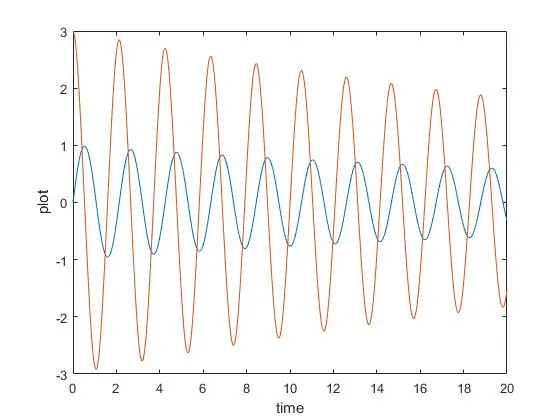
The plot showing the angular velocity and displacement the redline starting at 3 is the angular velocity and the blue line starting at 0 is the angular displacement. This plot is in the time span of 0 to 20 sec which is why the pendulum is not at rest by the end. Usage of better damping will result in the pendulum coming to rest by the end of 20 seconds.
Some of the errors I encountered while writing this program were
I tried using plot command instead of using the line command for plotting the pendulum but the color of the ball and the pendulum needed to be specified and I even thought of using a single plot command but realized that wouldn’t be possible because I can either combine two points or two lines but it is not possible to combine point and line in a single command. Eventually, with a little experimentation, I found my way out of these errors
CONCLUSION:
A graph representing the Angular velocity and displacement is plotted. In the video displaying the displacement of the pendulum it might seem that the ball is moving horizontally but upon zooming in it can be clearly seen that the ball is following a curvature. This is because of the small values of angles.
Links to the output videos
Notice that the amplitude of the pendulum is reducing with time.