Material Modeling from Raw Data in LS-Dyna
Objective: To model material data in LS-Dyna.
Procedure:
- The provided stress-strain curve image is imported into the data digitizer.
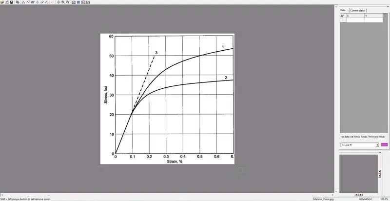
Fig 1: Stress-strain curve image is opened in the data digitizer to extract the curve points.
- From the data digitizer, the points from the 1st curve are exported into excel.
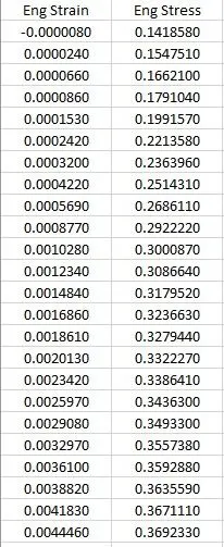
Fig 2: The stress and strain points are extracted from the image and exported in excel.
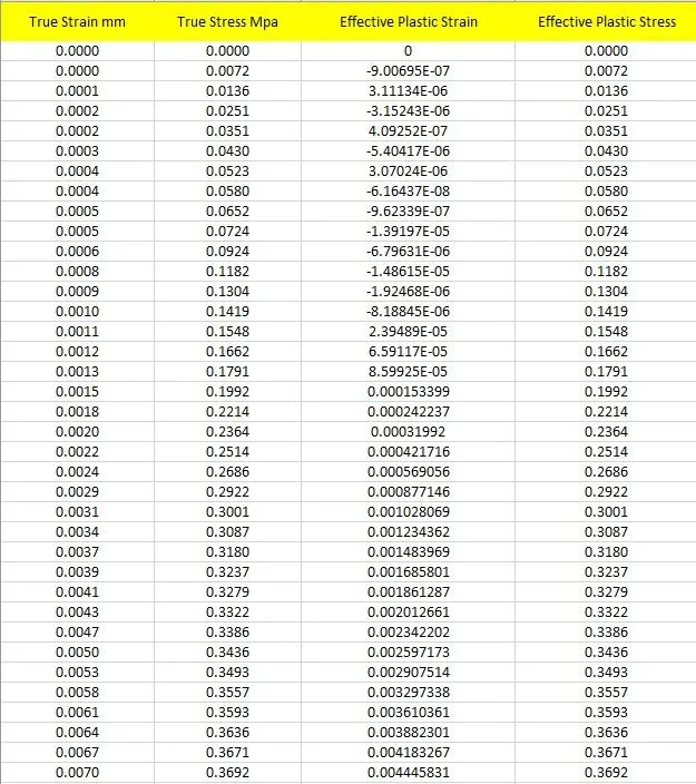
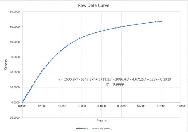
- The XY coordinates are saved in a suitable format for the LS-Dyna so that the file can be directly uploaded while the curve is defined.
- Open the given dog-bone specimen in LS-Prepost.
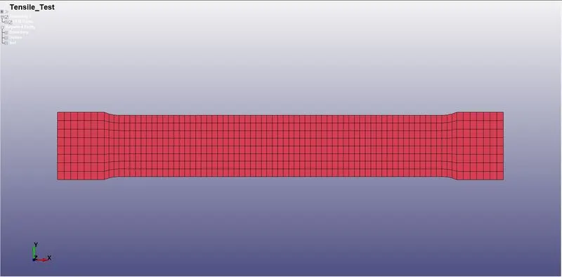
Fig 3: Dog-bone specimen.
- The initial keyword file contains the mesh information within it.
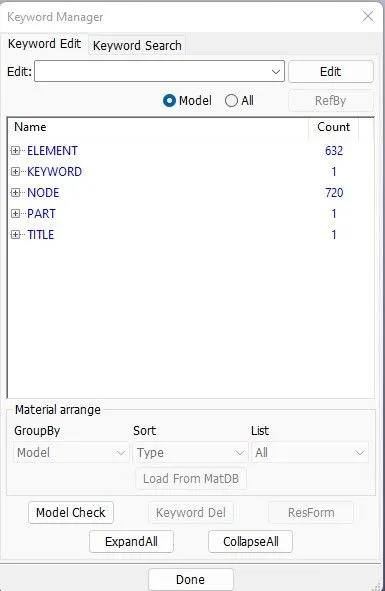
Fig 4: Initial keyword file.
- To completely define the keyword file, additional cards must be added to simulate the tensile test.
- The auto-created part is appropriately named for further identification.
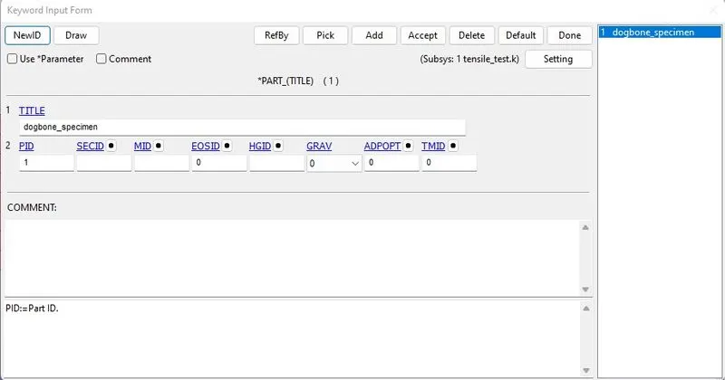
Fig 5: Part is appropriately named for later identification.
- A SHELL section card is defined with ELFORM=16 and a thickness of 2mm.
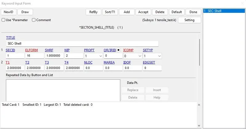
Fig 6: Shell section is defined with an ELFORM of 16.
- Hourglass card is defined to control the hourglass formation in the shell elements.
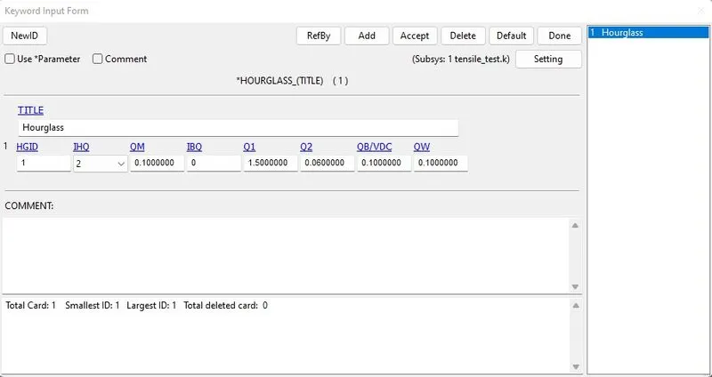
Fig 7: Hourglass is defined with Flanagan-Belytschko viscous form.
- Mat024 PIECEWISE_LINEAR_PLASTICITY card is defined with the following properties.
Density: 7.106e-06.
Young's Modulus: 144.10001.
Poisson's Ratio: 0.3000000.
yield stress: 0.1419000.
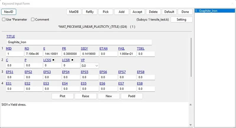
Fig 8: Mat024 card is defined.
- The curve taken earlier is now loaded into the curve card.
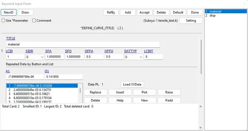
Fig 9: Stress-strain curve is loaded.
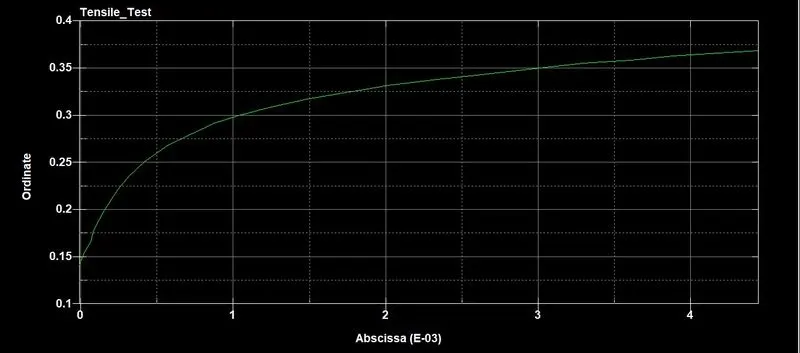
Fig 10: The curve is fed from the yield point.
- The displacement curve is also defined.
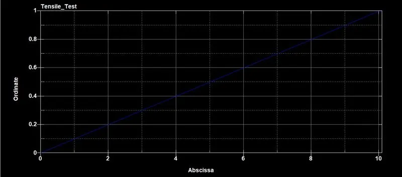
Fig 11: Displacement curve is defined up to the end of the simulation time.
- To emulate the tensile test for the specimen, a Single-point constraint is created with x translational and all rotational DOF fixed.
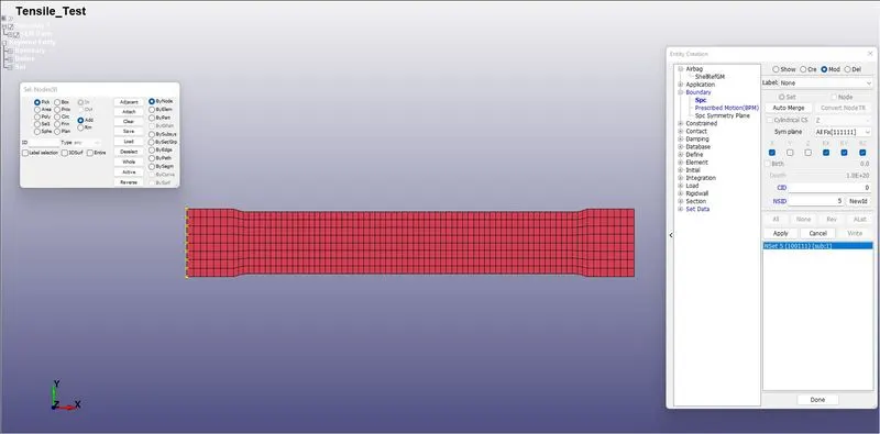
Fig 12: Left end of the specimen is fixed in x and all rotational directions.
- Additionally, y-translation is fixed on the mid node of the two ends of the specimen.
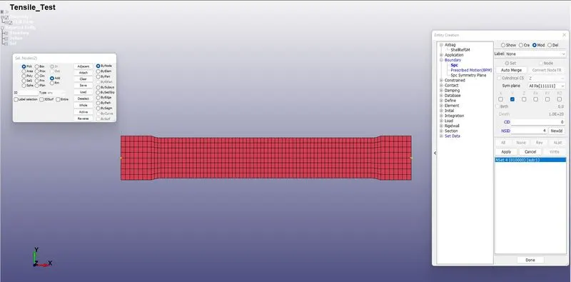
Fig 13: Mid nodes of the two sides are locked in y translational direction.
- A node-set is created with all the nodes from the right end of the specimen to provide displacement in the positive x-direction.
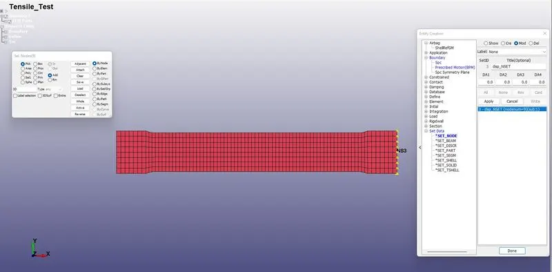
Fig 14: A node-set is created to define the displacement.
- Prescribed_motion_set is defined with the created node-set, and a DOF of 1 and VAD of 2 are chosen.
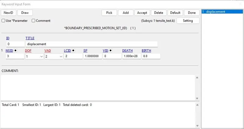
Fig 15: Displacement is defined to the other end of the specimen.
- To solve this particular simulation implicit solver is chosen. To define the implicit solver, specific implicit keywords must be included.
- IMPLICIT_AUTO, IMPLICIT_GENERAL, IMPLICIT_SOLUTION, and IMPLICIT_SOLVER keywords must be added from the control deck.
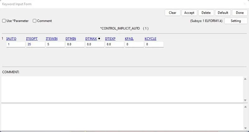
Fig 16: Implicit_auto card is defined.
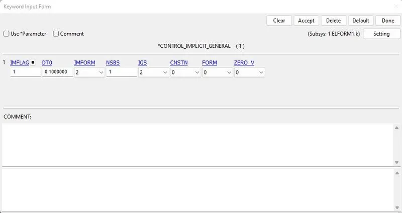
Fig 17: Implicit_general card is defined.
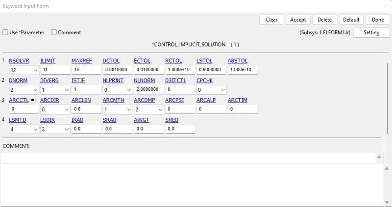
Fig 18: Implicit_solution card is defined.
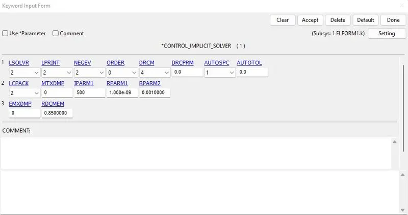
Fig 19: Implicit_solver card is defined.
- The ASCII_option keyword from the DATABASE deck is used for the output requests, and the GLSTAT option is checked.
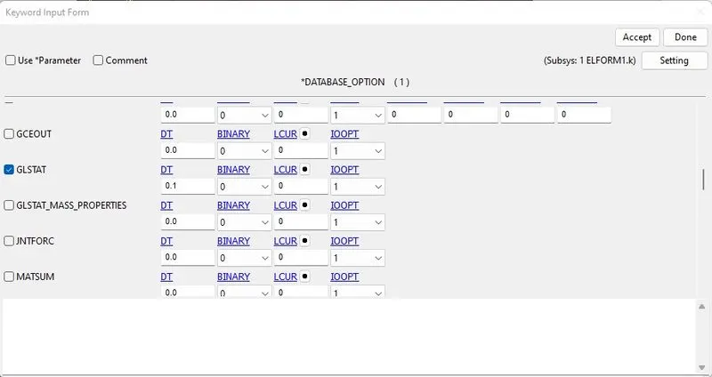
Fig 20: Output requests are defined.
- The BINARY_D3PLOT keyword from the DATABASE deck is used for the plots, and a DT of 0.05 is entered.
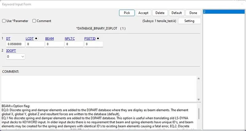
Fig 21: Plots at time intervals are defined.
- Finally, the TERMINATION keyword from the CONTROL deck is used to define the end time of the simulation.
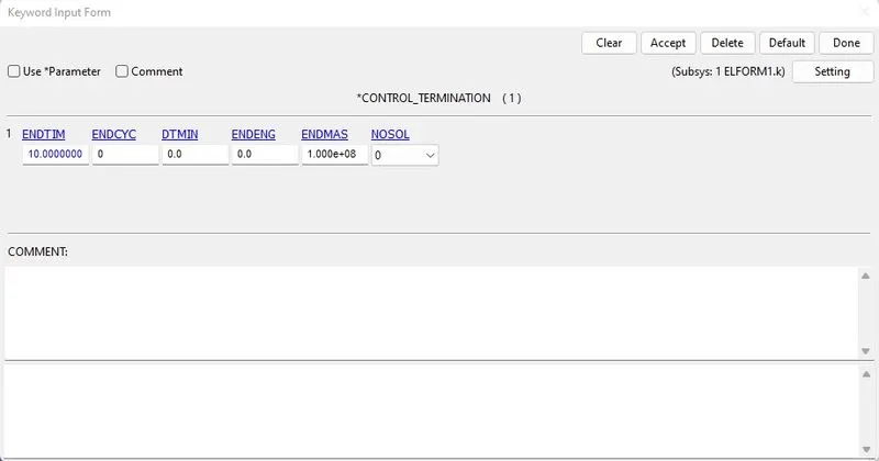
Fig 22: End time for the simulation is defined.
- With all these keywords included, the deck is fully defined and is now ready to solve.
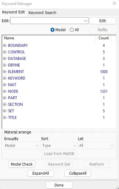
Fig 23: Fully defined deck.
- Open the Start LS-Dyna analysis, browse the keyword file, and hit run to run this keyword file.
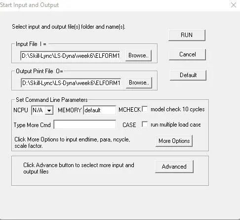
Fig 24: LS-Dyna analysis browser.
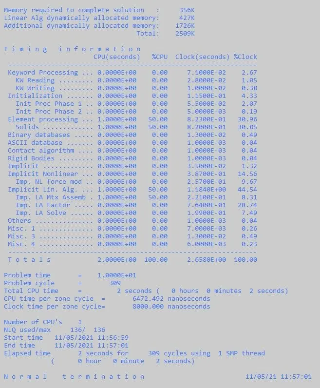
Fig 25: Successful completion of solving.
- Open new LS-PRE POST from the launch manager and open the LS-DYNA Binary plot (choose the D3PLOT file created) from the file menu.
- The model will be loaded the same as before, but we can access only the post-processing options from the right ribbon menu.
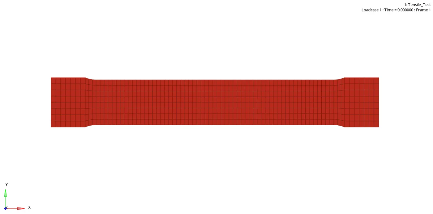
- The above animation represents the stretch in the specimen.
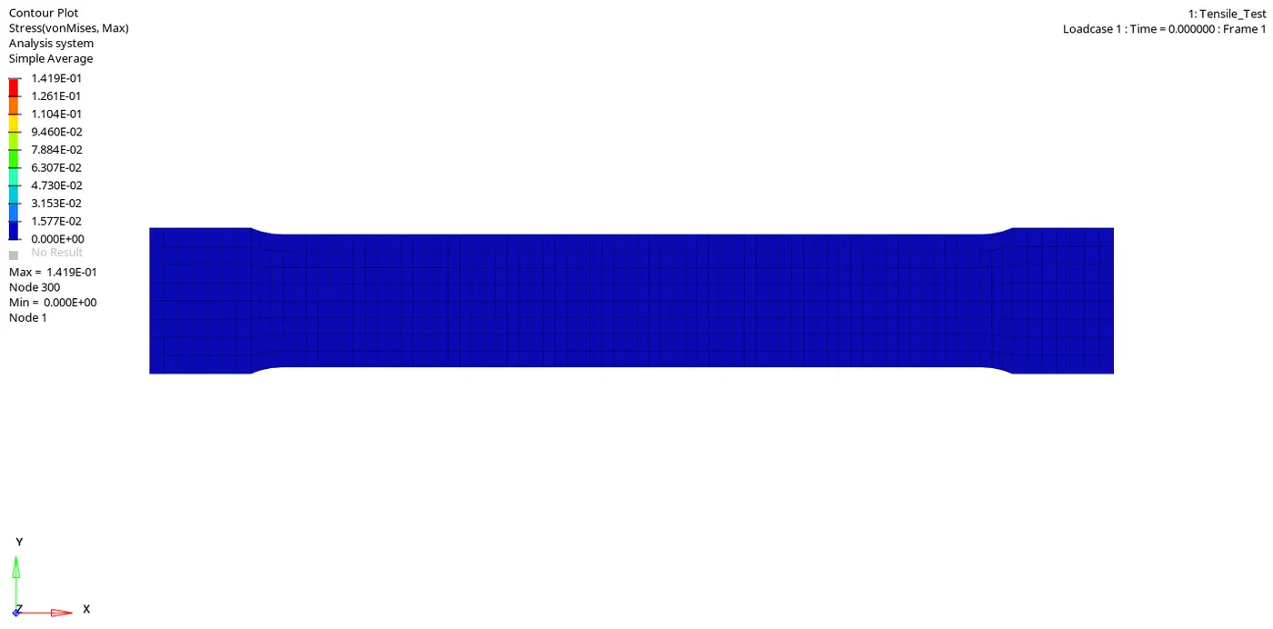
- The above animation represents the von mises stress in the specimen.
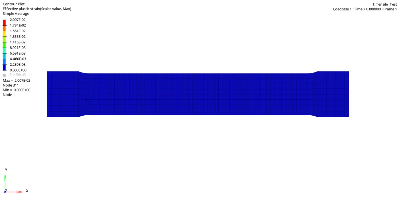
- The above animation represents the effective plastic strain in the specimen.
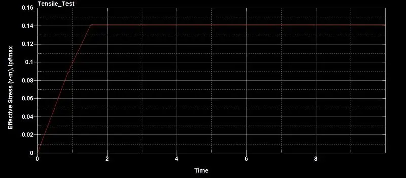
- The above graph represents the effective stress in the specimen.
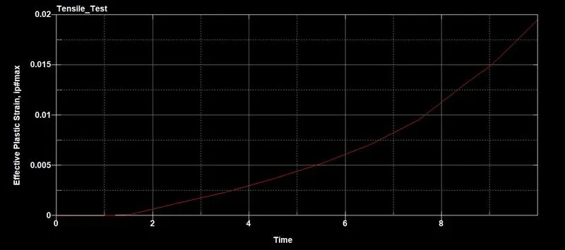
- The above graph represents the effective plastic strain in the specimen.
Conclusion:
Completed the process of modeling material in Ls-Dyna from the available test data and validated with the simulation result.