Week - 9 Material Modeling from Raw Data

AIM: To validate the MAT_24 material model using the given stress-strain curve.

Modelling Procedure:

Units: kg-mm-ms-KN-GPa

1. Data Extraction: Web Plot Digitizer was utilised to trace the coordinates from the given image. The methodology followed is depicted in the images.

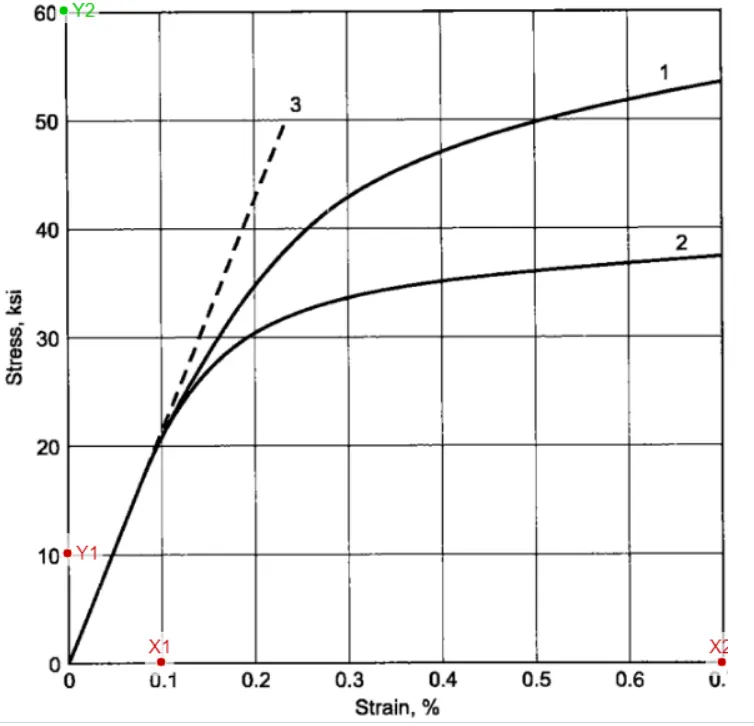
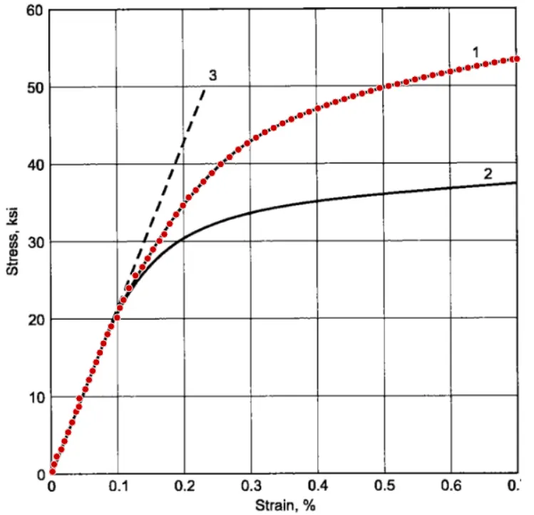
Fig: Axis alignment Fig: Manual Data Point Extraction

2. Unit Conversion:

Since for the simulation 'kg-mm-ms-KN-GPa' was followed, it was essential to maintain dimensional homogeneity. Thus, the stress was represented in terms of 'GPa' instead of 'ksi' and Strain was converted from percentage to dimensionless terms.

3. Data Cleanup and Curve Fitting:

The obtained coordinates were used to plot the curve and the polynomial equation of order 3 was used for curve fitting and an accuracy of 99% was obtained. Then a 0.2% offset line was drawn to determine the yield point of the curve and it was determined to be of 0.334GPa.

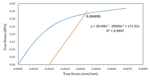
Fig: True Stress vs True Strain Plot with 0.2% offset line

4. Stress vs Strain Curve for Material Model:

Usually, the True stress vs True strain curve defines the material behaviour but experimentally, engineering stress vs engineering strain curve is obtained. Following relations can be utilised to convert the curve from engineering stress-strain to true stress-strain value.

True Strain = ln(1+Engineering Strain)

True Stress = (Engineering Stress)* exp(True Strain)

But to define the material properties in MAT 24 material model, the stress-strain curve needs to be defined in terms of Effective Stress vs Effective Plastic Strain. So,

Effective Plastic Strain = (Total true strain) - (True stress/E)

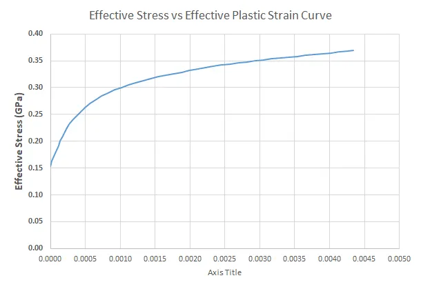
Fig: Effective Stress vs Effective Plastic Strain Curve

5. Numerical Modelling Methodology:

5.1 Material Model (MAT 24)

The given dogbone specimen was imported and the material properties were defined as follows:

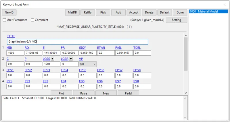
Material: Graphite Iron GJV 400 ( given material properties were found to be in a similar range)

Density: 7.1e-6 `(kg)/m^3`(literature)

Youngs Modulus: 144.1 GPa (Given)

Poisson's Ration: 0.26 ( literature)

Yield Stress: 0.153 GPa ( first stress value from the Load curve)

Failure: 0.004345 ( last strain value from the Load curve)

5.2 Element Formulation

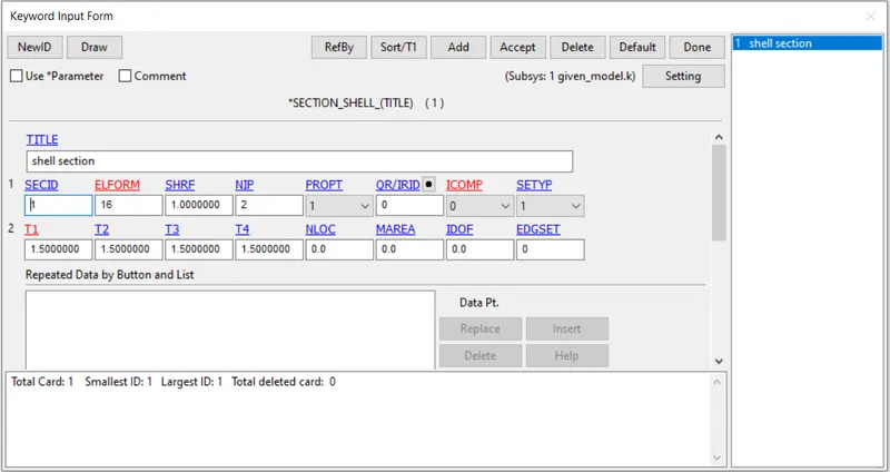
Fig: Element Formulation adopted for the simulation

5.3 Boundary Conditions

Fig: All the DOF was constrained except in Y-axis to facilitate the contraction of the material on application of tensile load.

Fig: A node-set was created to define the displacement motion to the model from another end.

Fig: Two central nodes along the s[ecimen were constrained in the Y-axis as it is known that there will be neither contraction nor expansion along the neutral axis of the specimen.

5.3 Control Conditions:

Implicit_Auto card - was included to automatically adjust the time step during the simulation.

Implicit_General - was defined to specify that the simulation is needed to be carried out using Implicit Formulation.

Implicit_Solution - the card was invoked to specify that a non-linear solution is expected as the simulation included plasticity and failure on the application of load.

Control_Energy - this card was included and HGEN was set to '2' so that Hourglass energy is calculated and included in the solution.

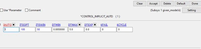
Fig: Control_Implicit_Auto Card

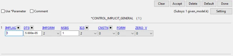
Fig: Control_Implicit_General Card

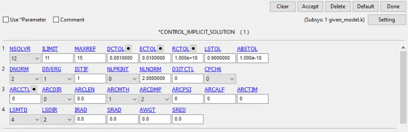
Fig: Control_Implicit_Solution Card

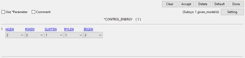
Fig: Control_Energy Card

6. Results and Discussion:

6.1 Effective Stress variation:

The effective stress variation is displayed were at a time of 0.8ms, failure is observed.

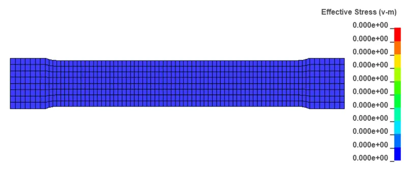
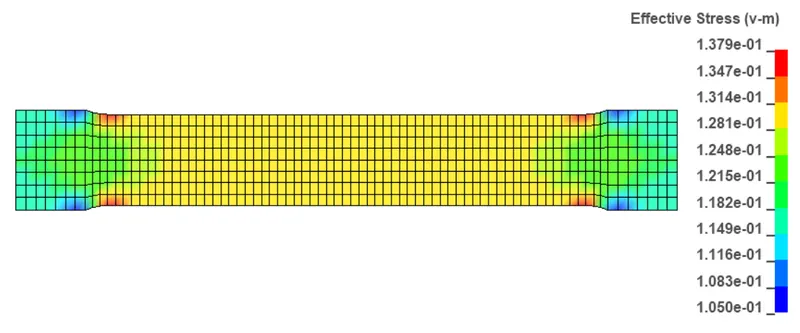
Fig : Effective Stress at t = 0.0ms Fig : Effective Stress at t = 0.126ms

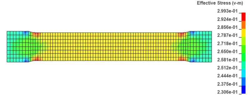
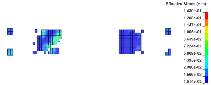
Fig : Effective Stress at t = 0.331ms Fig : Effective Stress at t = 0.846ms

6.2 Effective Plastic Strain variation:

'ELOUT' option was activated and the 'History_Shell' option was utilised to define an element at the centre of the given specimen. Also, 'STRFLG' was selected in the Extent_Binary card to obtain the effective plastic strain outputs.

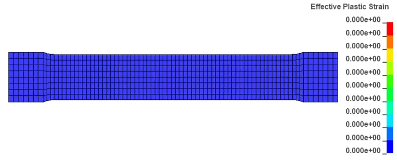
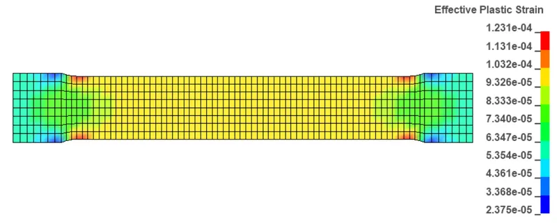
Fig : Effective Plastic Strain at t = 0.0ms Fig : Effective Plastic Strain at t = 0.206ms

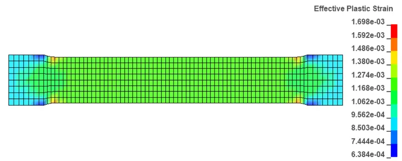
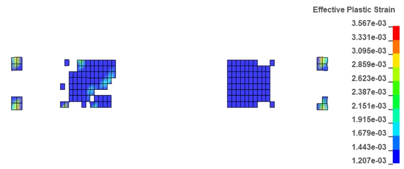
Fig : Effective Plastic Strain at t = 0.530ms Fig : Effective Plastic Strain at t = 0.846ms

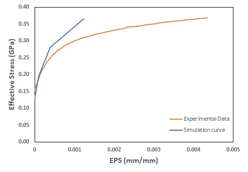
6.3 comparison of Stress vs Strain curve:

CONCLUSION

• Experimental Stress-Strain data and Numerical Stress-strain data are compared.
• The Simulation results over-predicts the experimental results which can be attributed to the fact that few of the material properties like density and poisons ratio were assumed from the literature.
• Different calibration processes like - mesh convergence and ELFORM can be tried to determine a solution closer to the experimental curve.
• The failure of the specimen is captured which is obtained about 0.846ms.