Week - 2 - Explicit and Implicit Analysis
Description of Implicit and Explicit Analysis
Introduction
Implicit and Explicit solvers are often used to solve dynamic problems, where the examples of dynamic problems are - nonlinear analysis, linear analysis like Modal and Force Response analysis.
Implicit analysis and Explicit analysis can be differentiated based on the time incrementation approach.
Implicit Analysis - Each time increment must converge while using this type of analysis; however, a relatively large time increment can be selected. The amount of the time step in implicit transient analysis has no intrinsic limit.
Explicit Analysis - Contrary to implicit analysis, in explicit analysis the time increment doesn't need to converge at every step, but smaller time increments are essential to obtain an accurate solution. In explicit analysis, the time step must be shorter than the time it takes a sound wave to traverse over an element.
AIM: To analyse the given function using Explicit and Implicit Methods and compare the outcome.
Explanation:
Given Data:
Considering the given function where the force 'f' is a nonlinear function of the displacement :
`f(u) = u^3 + 9u^2 + 4u`---(1)
then the stiffness 'k' as a fuction of displacement can be experssed by differentiating eq -1 w.r.t 'u' as :
`k(u) = (df)/(du) = 3u^2 + 18u +4`---(2)
Solving using Explicit Analysis
Using incremental explicit load control scheme, we have the following varaibles
displacement = u
displacement increment = `Delta u`
internal force = f
external applied force = F
Load Increment = `Delta F = 1``Delta F = k Delta u`
stiffness = k
STEP -1
`u_0 = 0.0`
then
`k(u_0) = 3(0^2) + 18(0) + 4 = 4`
considering incremental load = `Delta F_1 = 1`; we know that `Delta F = k Delta u`
So,
`Delta u_1 = (Delta F)/(k(u_0)) = (1/4) = 0.25`
`rArr u_1 = u_0 + Delta u_1 = 0 + 0.25 = 0.25`
`rArr f_i = (0.25^3) + 9 (0.25^2) + 4(0.25) = 1.578`
STEP -2
`u_1 = 0.25`
then
`k(u_1) = 3(0.25^2) + 18(0.25) + 4 = 8.687`
considering incremental load = `Delta F_2 = 1`; we know that `Delta F = k Delta u`
So,
`Delta u_2 = (Delta F)/(k(u_1)) = (1/8.687) = 0.115`
`rArr u_2 = u_1 + Delta u_2 = 0.25 + 0.115 = 0.365`
`rArr f_i = (0.365^3) + 9 (0.365^2) + 4(0.365) = 2.707`
STEP -3
`u_2 = 0.365`
then
`k(u_2) = 3(0.365^2) + 18(0.365) + 4 = 10.969`
considering incremental load = `Delta F_3 = 1`; we know that `Delta F = k Delta u`
So,
`Delta u_3 = (Delta F)/(k(u_2)) = (1/10.969) = 0.0911`
`rArr u_3 = u_2 + Delta u_3 = 0.365 + 0.0911 = 0.456`
`rArr f_i = (0.456^3) + 9 (0.456^2) + 4(0.456) = 3.790`
So, after the three iterations, the following result can be derived
`rArr F_e = Delta F_1 + Delta F_2 + Delta F_3 = 1 + 1 + 1 = 3`---(3)
`rArr f_i = (0.456^3) + 9 (0.456^2) + 4(0.456) = 3.790`---(4)
It is evident that the proposed system is not in equilibrium as `F_e ne f_i`
Summerising the Explicit Analysis Reuslts
| Step i | `Delta F_i` | `Delta u_i` | `u_i` | `(F_e)_i` | `(f_i)_i` | `(f_i)_i - (F_e)_i = R` |
| 1 | 1.0 | 0.25 | 0.25 | 1 | 1.578 | 0.578 |
| 2 | 1.0 | 0.115 | 0.365 | 2 | 2.707 | 0.707 |
| 3 | 1.0 | 0.0911 | 0.456 | 3 | 3.790 | 0.790 |
Solving using Implicit Analysis
The only difference that will be employed in the calculation is that at the end of each phase 'Newton-Raphson iterations are needed to be employed to obtain equilibrium and reduce the residual before moving to the next step.
STEP -1
`u_0 = 0.0`
then
`k(u_0) = 3(0^2) + 18(0) + 4 = 4`
considering incremental load = `Delta F_1 = 1`; we know that `Delta F = k Delta u`
So,
`Delta u_1 = (Delta F)/(k(u_0)) = (1/4) = 0.25`
`rArr u_1 = u_0 + Delta u_1 = 0 + 0.25 = 0.25`
`rArr f_i = (0.25^3) + 9 (0.25^2) + 4(0.25) = 1.578`
Checking the Residual
`rArr R^(o) = f_i - F_e = 1.578-1=0.578`
`||R^(o)|| > 10^(-2)`
thus, there is a need for Newton-Raphson iterations
Determining the correction `u_1 = u_1^(o)`
`delta u^1 = -[k(u_1^o)]^-1 R^o`
`k(u_1^o) = 3(0.25^2) + 18(0.25) + 4 = 8.687`
`delta u_1^1 = -(8.687)^-1 (0.578) = -0.066`
then, the updated value of displacement becomes
`rArr u_1^1 = u_1^o + delta u^1 = 0.25-0.066 = 0.183`
`rArr f_i = (0.183^3) + 9 (0.183^2) + 4(0.183) = 1.039`
Checking the Residual
`rArr R^(1) = f_i - F_e = 1.039-1=0.039`
`||R^(1)|| > 10^(-2)`
thus, there is a need for another Newton-Raphson iterations
`delta u^2 = delta u^1 - [k(u_1^o)]^-1 R^1`
`k(u_1^o) = 3(0.183^2) + 18(0.183) + 4 = 7.394`
`delta u_2^2 = -0.066 - (7.394)^-1 (0.039) = -0.071`
then, the updated value of displacement becomes
`rArr u_1^2 = u_1^o + delta u^2 = 0.25 - 0.071 = 0.178`
`rArr f_i = (0.178^3) + 9 (0.178^2) + 4(0.178) = 1.002`
Checking the Residual
`rArr R^(1) = f_i - F_e = 1.002 - 1 = 0.002`
`||R^(1)|| < 10^(-2)`
thus, no further iteration is necessary and the final value for the displacement at the end of STEP -1 is
`u_1 = 0.178`
STEP -2
`u_1 = 0.178`
then
`k(u_1) = 3(0.178^2) + 18(0.178) + 4 = 7.299`
considering incremental load = `Delta F_1 = 1`; we know that `Delta F = k Delta u`
So,
`Delta u_2 = (Delta F)/(k(u_1)) = (1/7.299) = 0.137`
`rArr u_2 = u_1 + Delta u_2 = 0.178 + 0.137 = 0.315`
`rArr f_i = (0.315^3) + 9 (0.315^2) + 4(0.315) = 2.184`
Checking the Residual
`rArr R^(o) = f_i - F_e = 0.184`
`||R^(o)|| > 10^(-2)`
thus, there is a need for Newton-Raphson iterations
Determining the correction `u_1 = u_1^(o)`
`delta u^2 = -[k(u_1^1)]^-1 R^o`
`k(u_2^o) = 3(0.315^2) + 18(0.315) + 4 = 9.967`
`delta u_2^1 = -(9.967)^-1 (0.184) = -0.018`
then, the updated value of displacement becomes
`rArr u_1^1 = u_1^o + delta u^1 = 0.315 - 0.018 = 0.297`
`rArr f_i = (0.297^3) + 9 (0.297^2) + 4(0.297) = 2.008`
Checking the Residual
`rArr R^(1) = f_i - F_e = 0.008`
`||R^(1)|| < 10^(-2)`
thus, no further iteration is necessary and the final value for the displacement at the end of STEP -2 is
`u_2 = 0.315`
Summerising the Implicit Analysis Reuslts
| Step i | `Delta F_i` | `u_i` | `(F_e)_i` | `(f_i)_i` | `(f_i)_i - (F_e)_i = R` |
| 1 | 1.0 | 0.177 | 1 | 0.995 | -4.493e-3 |
| 2 | 1.0 | 0.178 | 2 | 1.002 | 0.002 |
Discussion
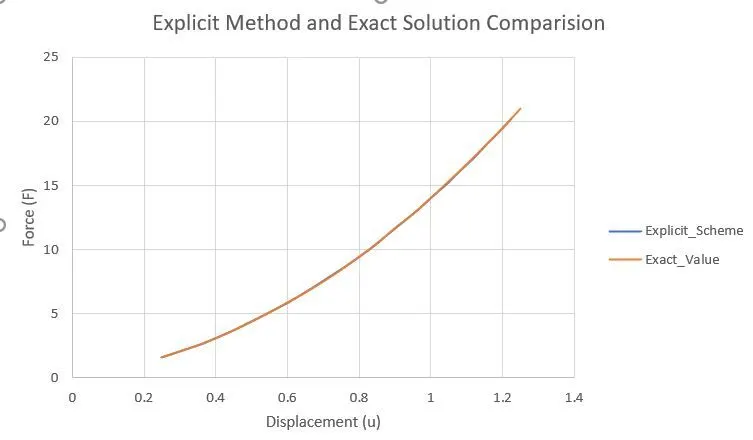
It can be observed from the graph that both explicit scheme and exact solution of the given system appear to predict appreciably acceptable results. Thus, it can be concluded that, since the differential equation has higher-order terms, the given problem can be solved using an explicit scheme.
Conclusion
Explicit and Implicit techniques are used to solve the given nonlinear equation. Each step in nonlinear implicit analysis necessitates a series of iterations to achieve equilibrium, within a particular tolerance. Iterations are not necessary for explicit analysis because the displacement is obtained directly. For the given system, both implicit and explicit method appears to produce accurate results where the implicit method appears to get the result quicker than the explicit scheme.