Week - 9 Material Modeling from Raw Data

Material Modelling

Objective

To derive the data from the given stress vs strain curve

Model the given tensile test specimen according to the derived data and compare the stress vs strain curves

Condition

- the elastic modulus is 20.9E+06 psi. or 114.1 GPa

- The units system to be used is kg-mm-ms

Theory

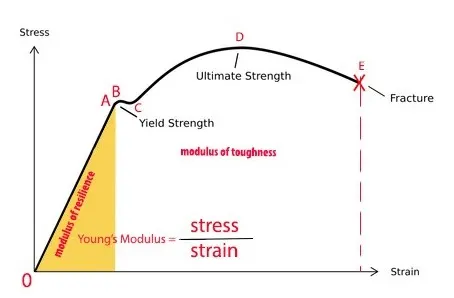
True strain = ln(1 + engineering strain) where ln designates the natural log

True stress = (engineering stress) * exp(true strain) = (engineering stress) * (1 + engineering strain) where exp(true strain) is 2.71 raised to the power of (true strain).

Be aware that experimental data always includes some degree of error and thus tends to be somewhat noisy or erratic. When using *MAT_24, one should input a smoothed stress-strain curve utilizing a minimal number of points. The input of noisy experimental data may cause spurious behaviour, particularly in the case of the default, 3-iteration plane stress plasticity algorithm for shells.

Effective Plastic Strain = Strain –

E=Youngs Modulus

Procedure

• Use Get Data Digitizer to derive the data from the graph.

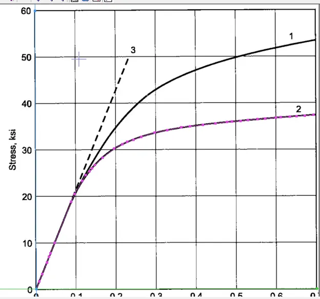
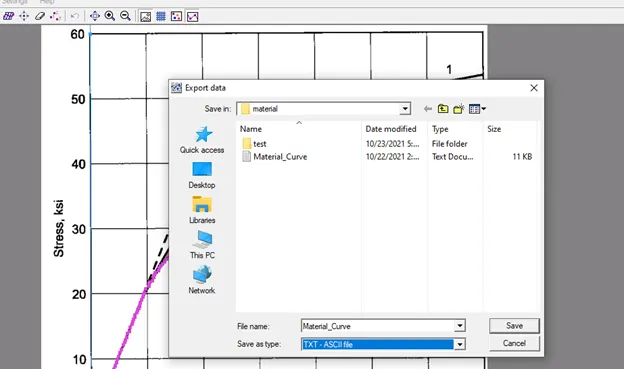
• Export this data in text format.

• Add the values of stress and strain in an excel sheet.

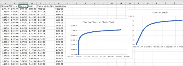
• Copy+Paste the values of Effective plastic Strain and respective stress above 0 in a new excel file.
• Save the file in a . CSV format.
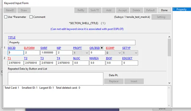
• After Importing the keyword file, we can start by creating the section shell card.

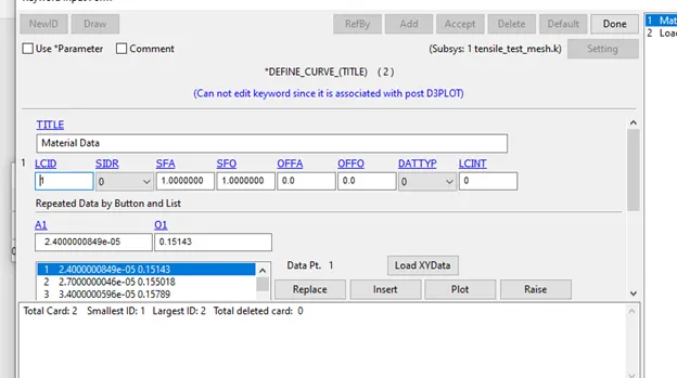
• Define the curve for material data.

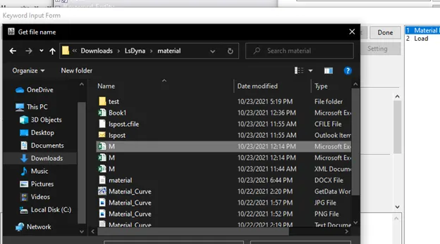
• Load X/Y data and select the .csv file created previously.

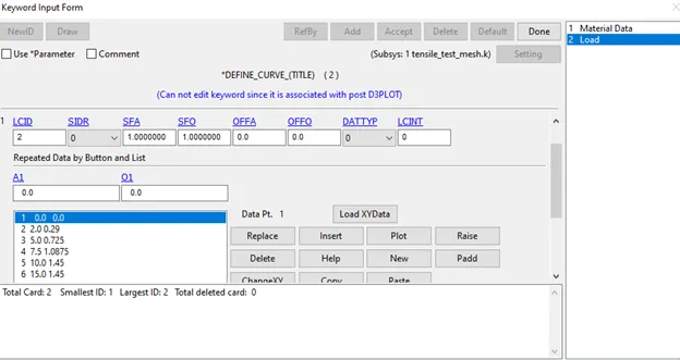
Define the Load Curve

• In keyword manager, go to define curve and plot the values appropriately for a linear increase.

• Stretch Ratio= exp(1+engineering strain)=exp(True Strain)
• Using the last value of strain,
• 01=1+engstrain
• 01=Final Length/initial Length
• 145*0.01=final length
  which gives us a value of 146.45mm as final length
• we can define the curve for 1.45mm displacement.

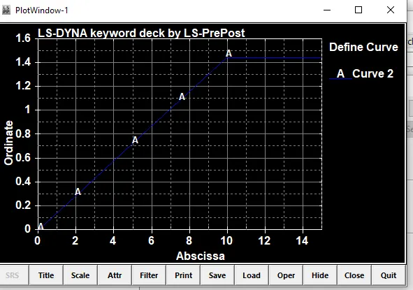
Material Data

• Create a mat24 card and add the values appropriately.

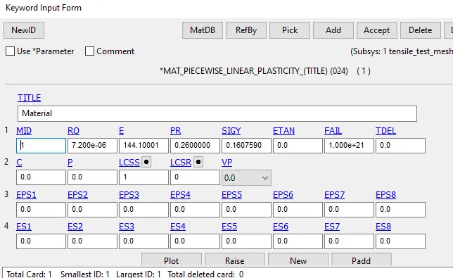
• Etan is ignored since LCSS is defined.

Boundary Conditions

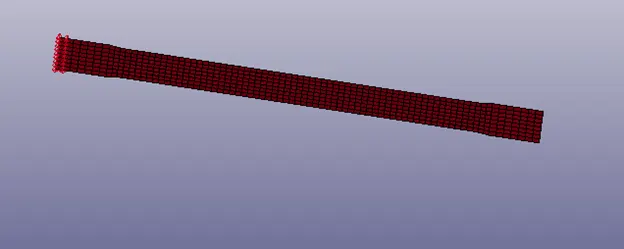
• Set the final layer of nodes on one side of the model as rigid on the x axis.

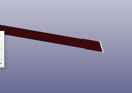
• For better stability, set the centre nodes of both side rigid on the y axis

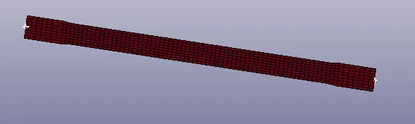
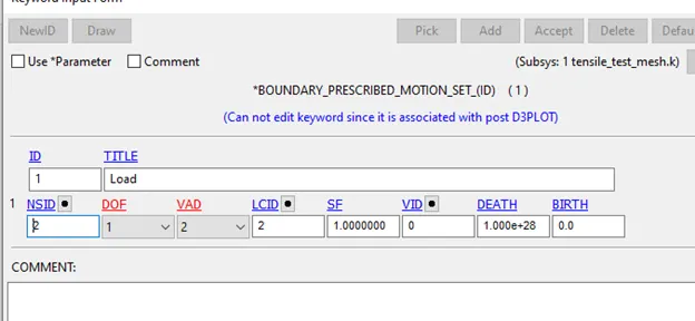
• After this,create a prescribed motion set for displacement.Set only the last layer of nodes opposite to the rigid ones for the Node Set Id.

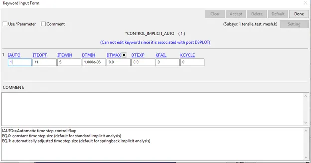
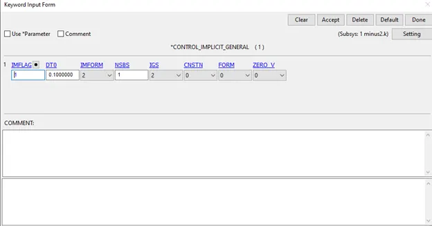
• Since the loading can be considered as Quasi Static , implicit solver can be chosen for this simulation and as such, implicit control keycards need to be created.
• It is recommended to go with the default properties for now

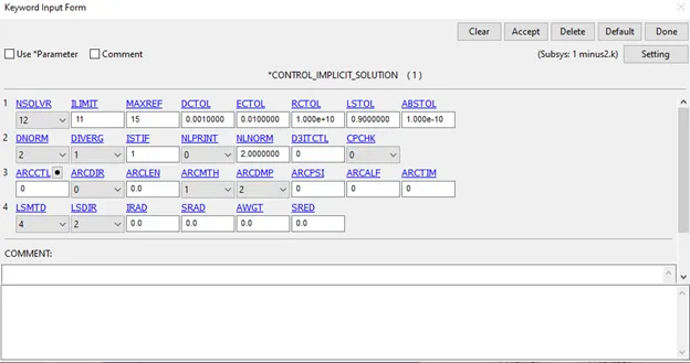
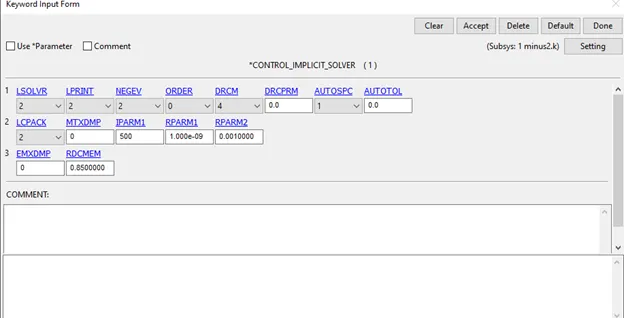
Output Files

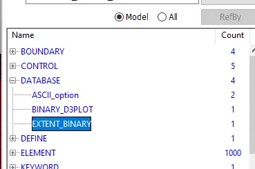
• In database, create the d3plot,extent binary and Ascii keywords

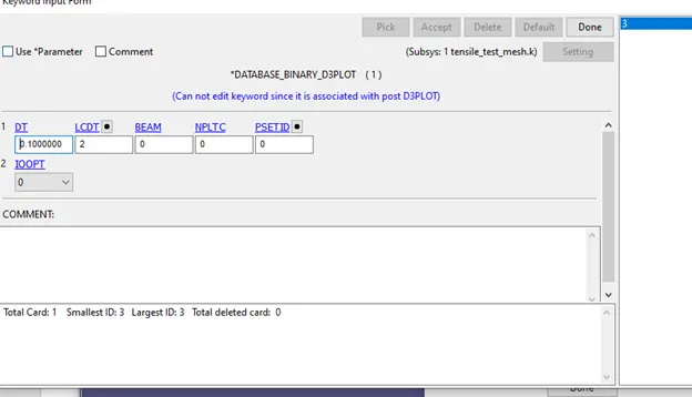
• In Ascii,enable Glstat and Matsum.

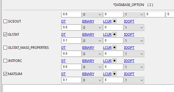
In extent Binary,set the values appropriately.

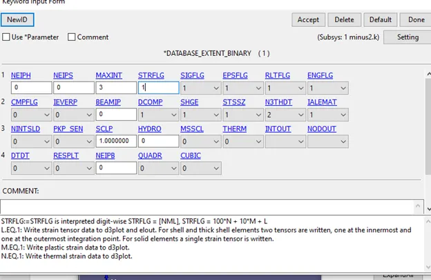
strflg is set to 1 to save the strain data.

Control

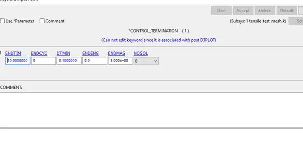
• Create a Control Termination Keyword

Check the keywords using the model checker for errors

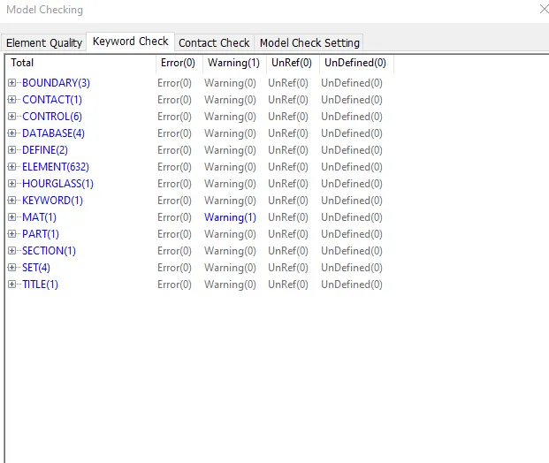
No errors only warnings

This could be due to an error while plotting from get data

After this run the simulation using the ls dyna solver

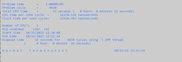
Make sure that the folder has no spaces and the termination is normal termination.

Post Processing

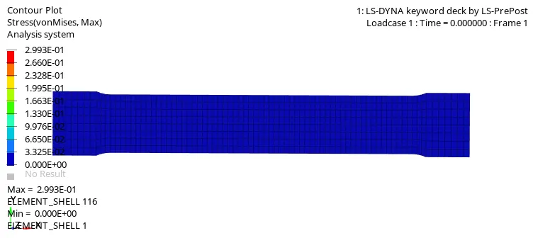
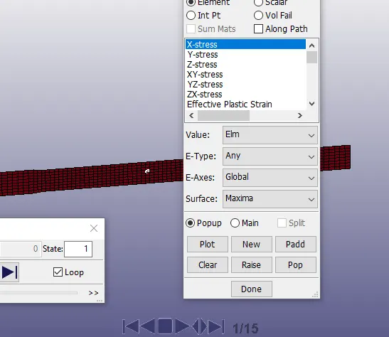
To get true stress and true strain values, in post go to history->element and plot X stress and Ipt Lower x strain.

After plotting, save the plot interpolating 20 points for the graph.

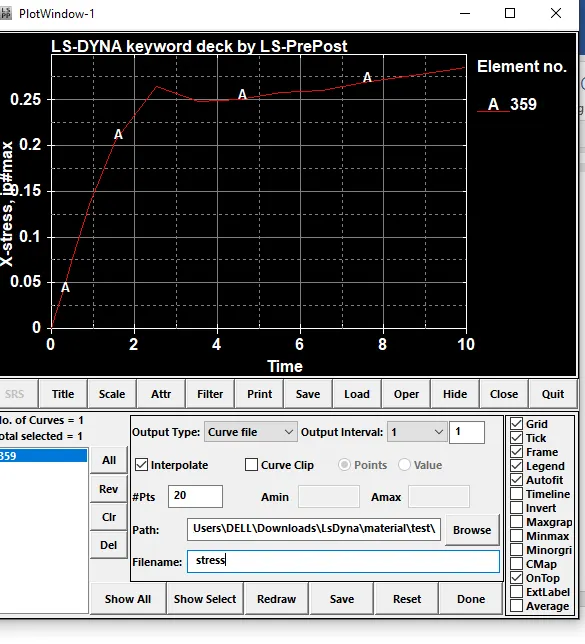
Do the same for true strain, plot lower IPT x strain.

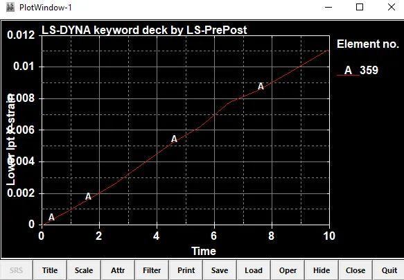
Open the files using notepad++.

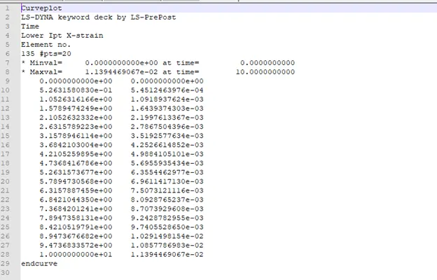
Plot them using excel.

Plot the Stress vs Strain graphs for the material data and simulation data.

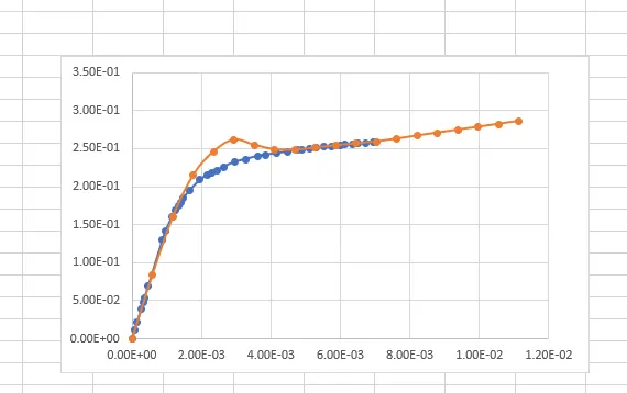
After plotting them , it can be observed that the linear portion of both graphs are similar.However, after the linear portion, there is a small difference in the graphs .This difference is due to the warning that states that slope is greater than youngs modulus.

This is an error in GetData Digitizer and can be recitified by adding more points in the region.

Learning Outcomes

• Implicit Analysis in Ls Dyna
• Cross plotting
• Material modelling in ls dyna

Conclusion

Material Modelling is an extremely important aspect of modelling an Fea simulation.

In this project, we modelled a graphite iron material model for a tensile test of a dogbone specimen.After plotting the stress-strain graph , it can be observed that the linear portion of both graphs are similar.However, after the linear portion, there is a small difference in the graphs .This difference is due to the warning that states that slope is greater than youngs modulus.The material data received from the graph has hence been validated.