Week - 9 Material Modeling from Raw Data

Aim-

By using the diagram of the true stress-strain curve of graphite iron casting. Two curves are there for different material structures. We need to pick any one of them and use the data to create either a MAT_024 or MAT_018 material model and then validate it.

Objective-

1. To extract the data from the diagram.
2. Clean the data and visually confirm that it matches the original data and the elastic modulus is 20.9E+06 psi.
3. Convert the data to (kg-mm-ms) unit system.
4. Process the data and create the material as demonstrated.
5. Use the material model with a dogbone specimen and validate the same.

Step 1: Extraction of data:-

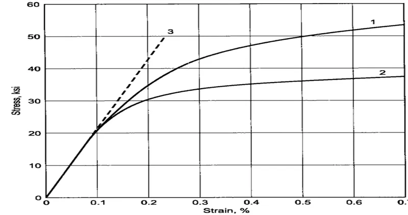
Procedure-

• As mentioned above we have to download the GetData Graph Digitizer software and then have to install it.
• Then we have to save the above image from .png to .jpg format, as it is only acceptable file format in graph digitizer.
• Now we have to create the co-ordinate axes and then set the data as per graph then we have to start selecting the point accoringly.

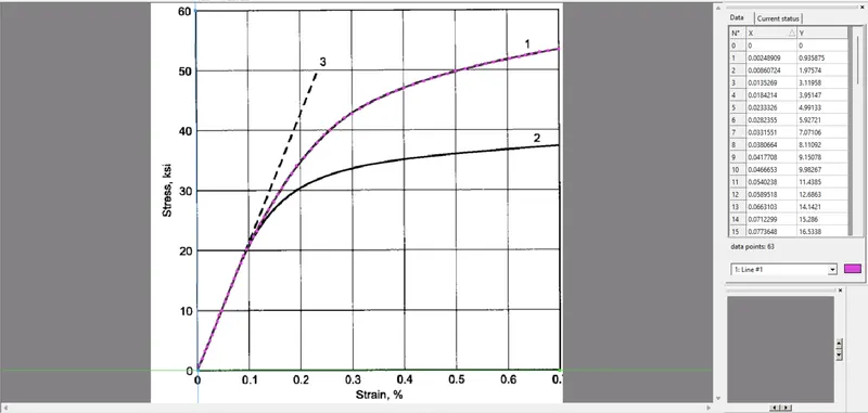
• From above snap we can observe that, I have selected curve no.1 in graph.
• Now we will export this table date to .xls format to start getting the input values accordingly.
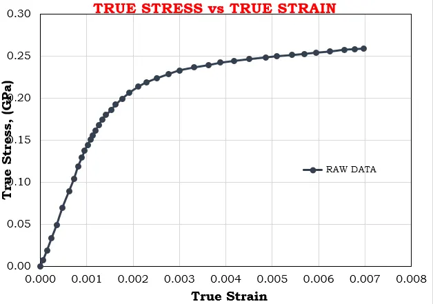
• Now we will open the excel file and do the calclulations.

Step 2: Model setup in LS Dyna:-

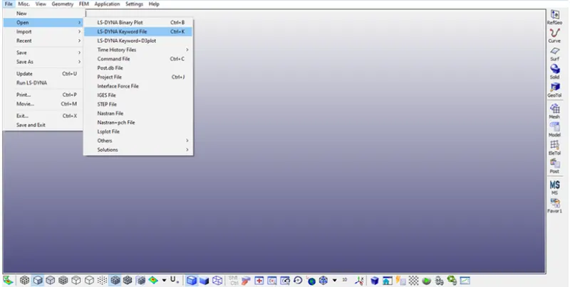
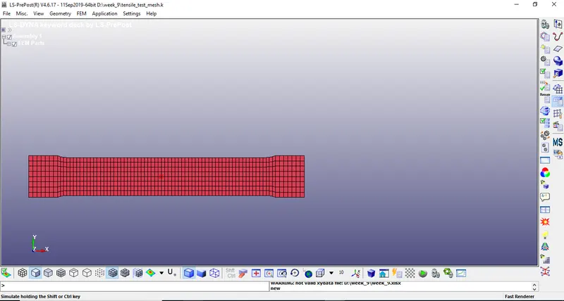
• We have to open the given LS-Dyna keyword (.k file) file in LS-PrePost, using option File>Open>LS-Dyna Keyword File as shown in below snap.

Step 3:-Creat Section_sell:-

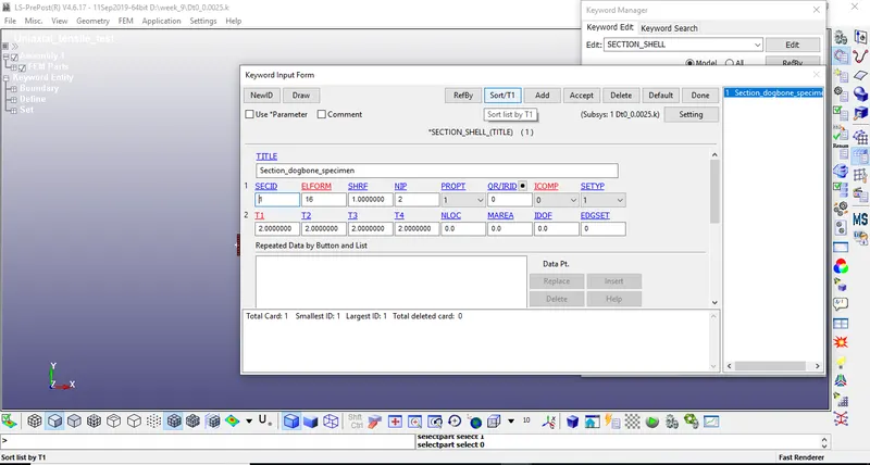
The dogbone specimen is defined with shell elements of thickness 2mm and ELFORM 16 as shown below.

Step 4:- Creat Curve :-

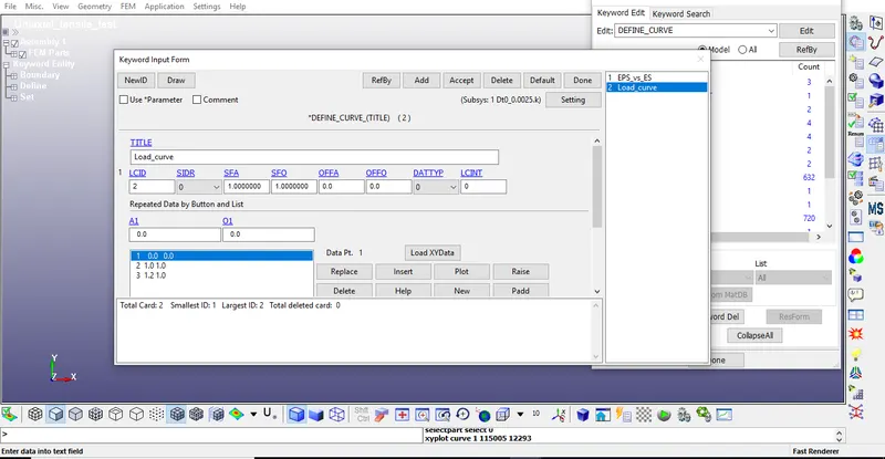
• Now we will go to the Define>>curve and input the value of curve data to get the curve.

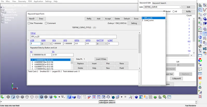
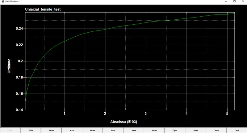
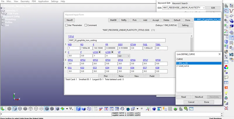
• The LCSS contains the load curve of effective plastic strain EPS vs effective (true) stress ES.

  The effective plastic strain is calculated in the excel sheet from the true stress value using the relation

  Effective plastic strain = True strain - (True stress/ Young's modulus)

  The region of the curve after the yield point (144 Gpa) is the plastic part of the curve. Therefore the values in the excel sheet after this stress point, and the corresponding EPS values are input into LS Dyna and the curve is generated as shown below.

LCSS :-

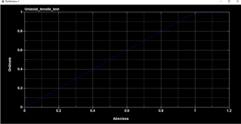
Prescribed Motion Curve:-

Step 5:- Create the MAT card for it as MAT24_PIECEWISE_LINEAR_PLASTICITY.

Material Definition

The MAT 24 piecewise linear card is defined with the following parameters. The unit system used is kg-mm-ms. The Young's modulus (E) is 20.9 e+6 psi which is 144.100 Gpa. The value of density (RO) and poisson's ratio (PR) are given accordingly.

Part Creat:-

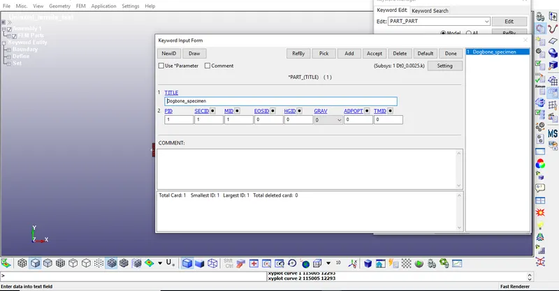
Finally we have to assign the section and material to the part.

Step 6:-Creat Boundry Condition:-

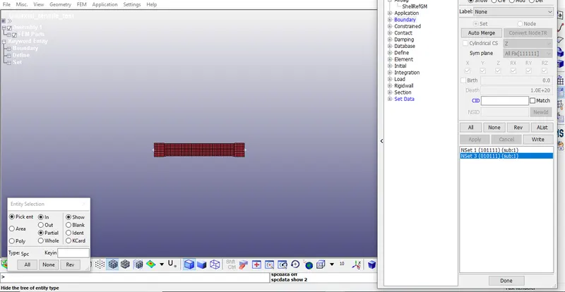
SPC:-

The nodes on the left edge of the specimen and constrained in the X and Z directions. They are not constrained in the Y - direction, since the speciment undergoes lateral elongation during the test.

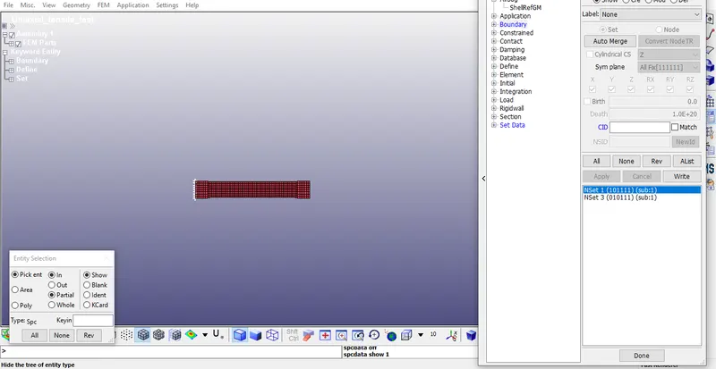
The middle nodes on either edge are constrained in the Y - direction

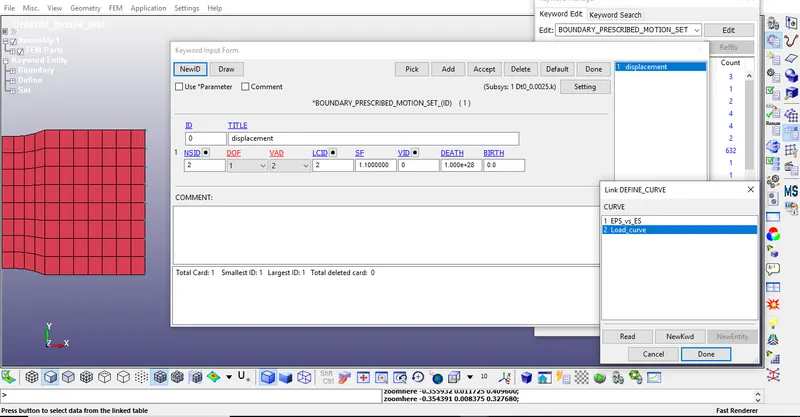
PRISCRIBED MOTION SET:-

A displacement is given to the nodes at the right edge of the specimen as shown below.

Step 7:- Creat Database and Control cards:-

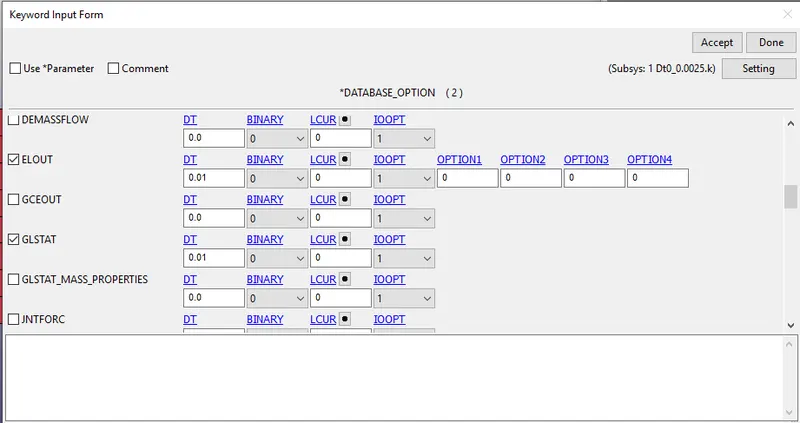
The database cards are defined as shown below.

The timestep for BINARY_D3PLOT and DATABASE_ASCII for GLSTAT and ELOUT are 0.1 ms.

DATABASE_EXTENT_BINARY card with STRFLG = 1 is used to compute the elastic strain in the model.

Control_terminetion:-

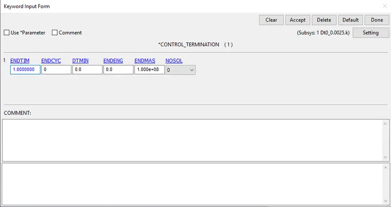
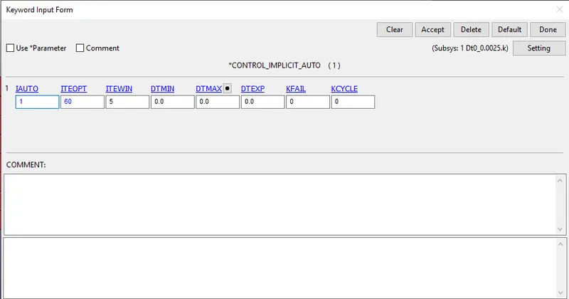
Control_Implicit_Auto:-

Control_Implicit_General:-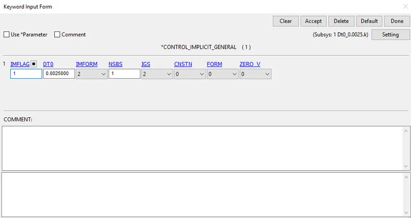

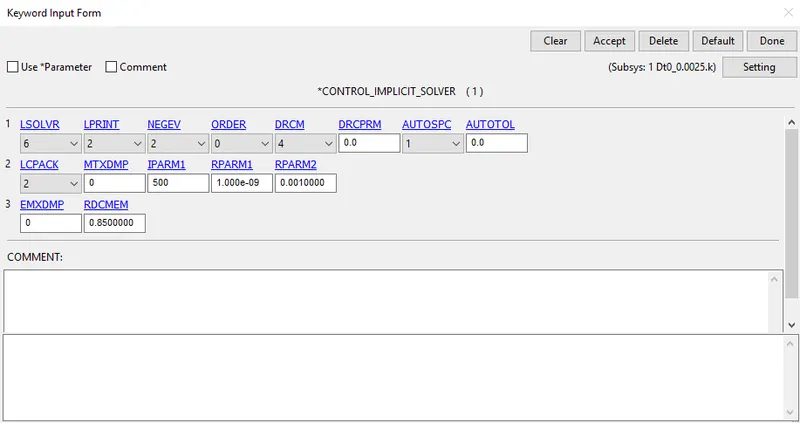
Control_Implicit_Solver:-

DataBase:-

• Now we will create the database file.
• BINARY_D3PLOT - It defines the frequency at which the animation file is to be created and is set to 0.01ms.
• Extent Bianry database card.

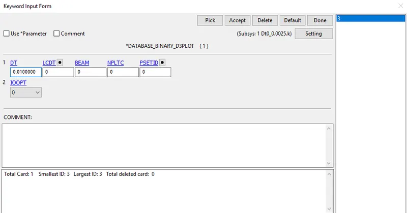
The output request in ASCII format, The following keyword are activated

1. ELOUT-Element Output Data
2. GLSTAT- Global Data
3. MATSUM- Material Energies and
4. RCFORC: Resultant Interface Forces

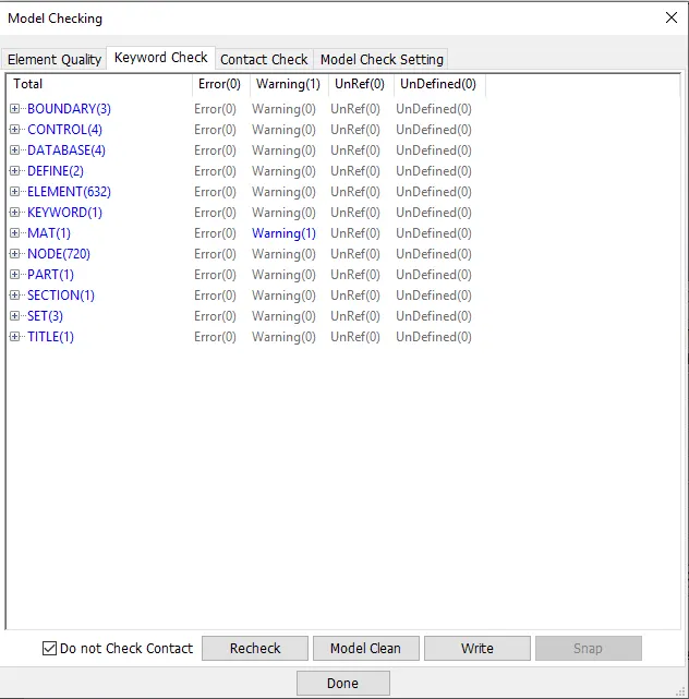
• Now we will check the model and then head for simulation.

RESULTS:-

• Since there is no error we can proceed further to save and run the keyword file.

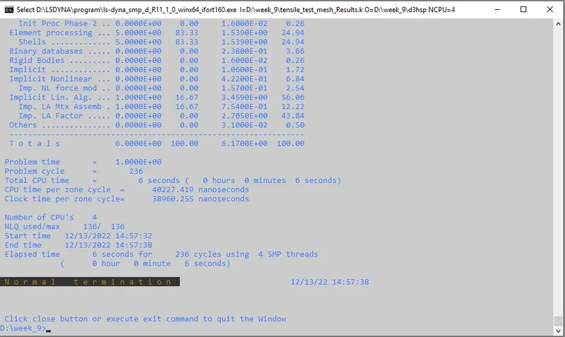
• As simulation ended with Normal Termination. Therefore, the model is simulated successfully.
• Now we can open this files one by one using LS-post processor.

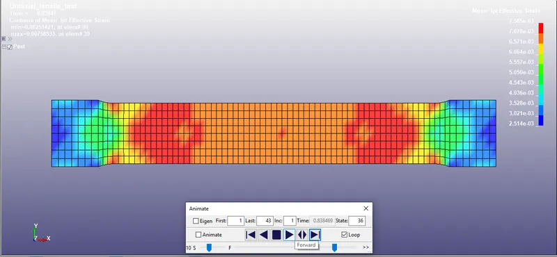
Results & Plots-

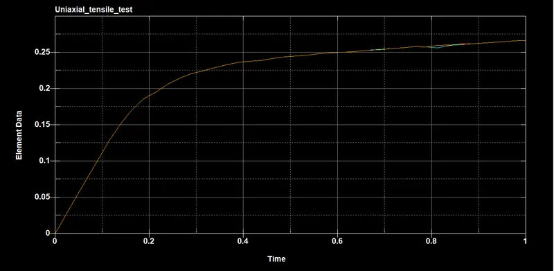
Effective Stress (V-M)-

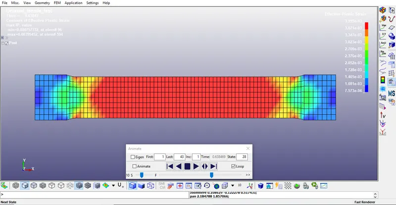
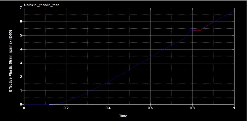
Effective Plastic Strain-

Plots-

Effective Stress (V-M)-

Effective Plastic Strain-

Now Effective Stress Vs Effective Plastic Strain-

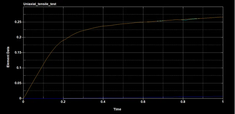
From above data we can observe that the graph values, calculated values and simulated values are almost equal to we can say that our material model is correct.

Animations-

The animation of the von mises stress can be seen below.

The maximum stress is 0.2709 GPA, which is higher than the yield strength limit off 144 GPA. This means that plastic deformation occurs in the material. Necking, however, has not yet been develeoped.

The peak effective plastic strain is 0.00756.

Conclusion:-

• The stress-strain data extracted from the image is validated with the MAT_024(Piecewise linear plasticity) material model.
• The stress-strain behaviour after yielding is considered by a hardening curve which is given as an input through the MAT_024 card.
• The MAT_024 material model captures the actual stress-strain behaviour similarly and almost matched the defined stress-strain curve in the material model.
• Also we have seen little variation in the simulation data, which can due to the lack of information like density and Poisson’s ratio for the raw data, Mesh Size of the model or defining proper strain rate. These variations can be fine-tuned by trying different values of these properties and by selecting more data points to better capture the curve feature.