Week - 9 Material Modeling from Raw Data

AIM
The main aim of this challenge is to understand how to model a material from raw data which is obtained from lab tests and also to validate it at the end so as to make sure that a correct material model is created which can then be used for different kinds of simulations.

EXPLANATION

In this challenge we are provided with the image of true stress vs strain percent curve of a graphite iron casting. We need to create *PIECEWISE_LINEAR_PLASTICITY material model from this data and then validate the same. Usually a specimen of required material is tested in a lab so as to get the stress and strain values. Suitable material model is then used so as to get the desired material behaviour. The values that we input in the material model card should be in correct format and also a simple test like a tensile test on a dogbone specimen should be done so as to check if there is any error or deviation from the input values before giving the material model to a complex part or set of parts.

CASE SETUP
To extract the strain percentage and true stress values from the image given, we use a data digitizer tool. Here we are using the 2nd graph in the image for our purpose. We need at least 50-100 data points for inputting in the material model. After collecting the data points from the graph, it is exported into an excel file. From there, the strain percentage values are converted to true strain values. This is done by diving the strain percentage by 100 i.e true strain = strain percent /100. After this the true stress values which are obtained in Ksi (kilo pound per square inch ) is converted to kg-mm-ms units using the conversion factor 1Ksi = 0.006895 kg/mm (ms)2.

The Young's modulus of the graphite iron casting is found by calculating the slope of the true stress vs true strain curve. We find this by using the SLOPE function in excel and using the first twenty eight values. The young's modulus was then found to be E=144.4182175 kg/mm(ms)^2. In *MAT_024 the material data has to be given in terms of true stress and effective plastic strains as LS-DYNA can easily calculate the linear portion of the curve using the youngs modulus value. For finding effective plastic strain we use the formulae, effective plastic strain = total true strain - (true stress/youngs modulus).

For finding the yield strength from the data we use the 0.2% offset strain method. Here we 1st find 0.2% offset strain values from the true strain values we have found out i.e (0.2 %offset strian= true strain +0.002). Similarly we find the 0.2% offset stress using the formulae , 0.2% offset stress = true stress* youngs modulus. Now we plot these offset stress and strain values in the same graph containing the true stress and true strain plot. The intersection point of these two graphs will yield the yield strength.The yield strength was found to be 0.2487928. The graph plotted to find yield strength is shown below.

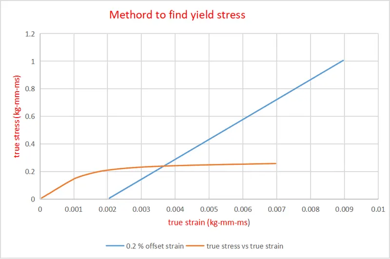
Thus we have found out the necessary parameters for creating our material model from our input data. Now, we need to validate the material model so as to find any errors or discrepancies. For this we will use the material model we have created to run a simple tensile test on a dogbone specimen and then check whether the output stress vs strain plot obtained matches with our input stress-strain values.

We import a dogbone specimen keyword file that we have on to LS-Prepost. In our case we have a simple 2D dogbone specimen. The 1st step is to arrest all DOF except translational degree of freedom in the x-direction of the neutral axis using *SPC_SET keyword . The next step is to constrain the nodes at the end of the specimen in all directions except translation in y direction.For giving displacement to the specimen we need to first define a load curve. For this we use *DEFINE_CURVE keyword. A load curve with a maximum displacement of 1.015mm (max strain* length of specimen) is defined.

*PRESCRIBED_MOTION_SET keyword is used to give the required displacement in the x-direction and the displacement is given to the nodes at the end of the specimen.

*DEFINE_CURVE keyword is used to input the true stress vs effective plastic strain curve into LS-DYNA.

Now, the material model is created using * MAT_024 (MAT_PIECEWISE_LINEAR_PLASTICITY ) card. The young's modulus, E= 144.4182, RO= 7.3e-06, SIGY= 0.2487928, PR=0.31 are entered. The true stress vs effective plastic strain values which we have defined earlier in * DEFINE_CURVE is input in the LCSS option. *SECTION_SHELL is used to define the section of the specimen with t1=1.0mm.

*PART_PART is used to give the correct section and material to the specimen.
*CONTROL_TERMINATION is used to give a termination time of 1ms.
*DATABASE-BINARY_D3PLOT is activated with DT=0.1. *DATABASE_ASCII_option is used to activate GLSTAT and MATSUM with DT= 0.1.

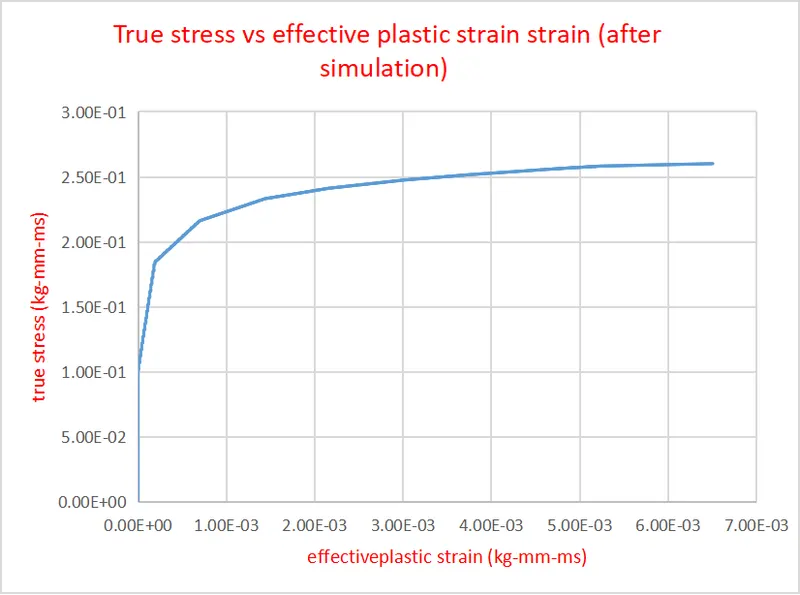
The simulation is then run and the output true stress vs effective plastic strain plot is taken from the post processor to compare it to the input values.

RESULT

The true stress vs effective plastic strain values obtained after simulation is shown below.

The input true stress vs effective plastic strain plot is shown below.

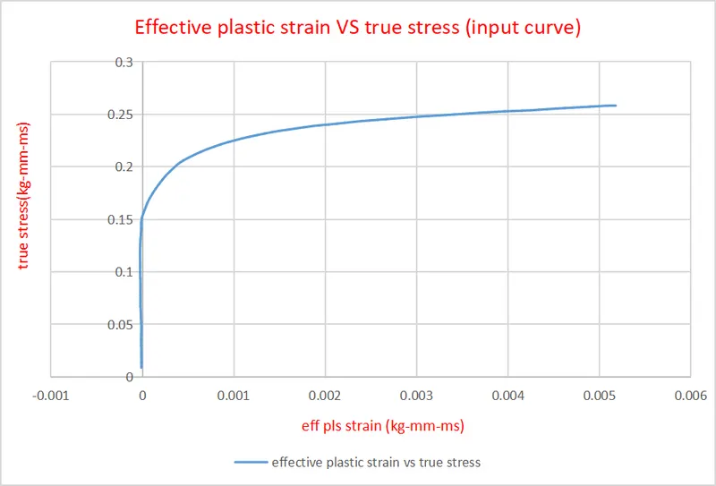
When comparing the two input and output graphs we find that they are very similar. Hence our material model can be used in other simulations without any fear.