Week 11 - Simulation of Flow through a pipe in OpenFoam

Simulation of Flow through a pipe in OpenFoam

Objective:

The main objective of this challenge is to simulate an axi-symmetric flow by applying the wedge boundary condition and to validate your results with the Hagen- Poiseuille's equations for the fully developed flow. Another objective is to write matlab code to generate blockMeshDict file automatically.

To start the challenge, initially we need to assume certain things:

a) The flow is laminar and flows through a constant cross-section pipe at an inlet Reynold's number of 2100. Generally for the laminar types of flows, we will use icoFoam solver in openFoam.

b) The diameter of the pipe as 0.02m ( by choosing small diameters, the simulation will execute fastly.)

As we assumed diameter of the pipe as, d = 0.02m

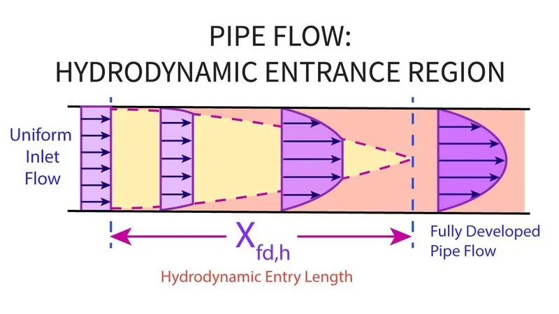
As the flow is laminar Entry Lengths The hydrodynamic entry length is usually taken to be the distance from the pipe entrance to where the wall shear stress (and thus the friction factor) reaches within about 2 percent of the fully developed value. In laminar flow, the hydrodynamic entry length is given approximately as

L_e = 0.06*Re*d

To validate the results with Hagen Poiseuille's law, the following data for standard water has to be known

diameter, d = 0.02m

radius,r = d/2 = 0.01m

length at entrance, L_e = 0.06*Re*d

length at exit, L_t = L_e + 0.25*L_e (As the lenght of the pipe at exit is definitely longer than at entry, consider it as 25% of entrance length)

dyanamic viscocity, mu = 0.00089 N/m^2

density, rho = 997 kg/m^3

Reynolds number, Re = 2100

kinematic Viscocity, nu = mu/rho

Hagen - Posieuille equation:

n nonideal fluid dynamics, the Hagen–Poiseuille equation, also known as the Hagen–Poiseuille law, Poiseuille law or Poiseuille equation, is a physical law that gives the pressure drop in an in compressible and Newtonian fluid in laminar flow flowing through a long cylindrical pipe of constant cross section.

The assumptions of the equation are that the fluid is incompressible and Newtonian the flow is laminar through a pipe of constant circular cross-section that is substantially longer than its diameter; and there is no accelaration of fluid in the pipe. For velocities and pipe diameters above a threshold, actual fluid flow is not laminar but turbulent, leading to larger pressure drops than calculated by the Hagen–Poiseuille equation.

Equations for hagen poiseuille are:

Average Velocity, V_a = Re*mu/ rho* d

Maximum Velocity, V_m = 2*V_a

Pressure difference, delta_p = 8*mu*L_t*v_a/ r^2

Kinematic Pressure, P_kin = delta_p/ rho ( As the pressure comes from above equation will be in pascals, so we are using kinematic pressure)

Shear stress, tau = 2*mu*V_m*r/ r^2

As the data is ready, first we write code im Matlab to generate automatic blockMeshDict file and it will be as follow:

clear all
close all
clc

%Initial Data
d = 0.02; %diameter of the pipe
r = d/2;  % radius of the pipe
Re = 2100;
L_e = 0.06*d*Re; % length of the pipe at entrance
L_t = L_e+0.25*L_e; % total length of the pipe
theta = input('Enter the value of wedge angle =') %Angle of the wedge;
mu = 0.00089; % Dyanamic viscosity of the water
rho = 997;  %density of water
nu = mu/rho;   % kinematic viscosity
%average velocity of the water in the pipe
v_a = (Re*nu)/d;
% maximum velocity of the waterfall
v_m = 2*v_a;
%pressure gradient across the pipe
delta_p = (8*mu*L_t*v_a)/(r^2);
%kinematic pressure
kin_p = delta_p/rho;

%% Scrpit for blockMeshDict

header1 = '/*--------------------------------*- C++ -*----------------------------------*\'
header2 = '=========                 |'
header3 = '\\      /  F ield         | OpenFOAM: The Open Source CFD Toolbox'
header4 = ' \\    /   O peration     | Website:  https://openfoam.org'
header5 = '  \\  /    A nd           | Version:  8'
header6 = '   \\/     M anipulation  |'
header7 = '\*---------------------------------------------------------------------------*/'

f1 = fopen( 'blockMeshDict.txt','w');
fprintf ( f1, '%s\n', header1);
fprintf ( f1, '%s\n', header2);
fprintf ( f1, '%s\n', header3);
fprintf ( f1, '%s\n', header4);
fprintf ( f1, '%s\n', header5);
fprintf ( f1, '%s\n', header6);
fprintf ( f1, '%s\n', header7);

fprintf (f1, 'FoamFile\n');
fprintf (f1, '{\n');
fprintf (f1, '%12s \t 2.0;\n', 'version');
fprintf (f1, '%12s \t ascii;\n', 'format');
fprintf (f1, '%12s \t dictionary;\n', 'class');
fprintf (f1, '%12s \t blockMeshDict;\n', 'object');
fprintf (f1, '}\n');
fprintf ( f1, '%s\n\n', '// * * * * * * * * * * * * * * * * * * * * * * * * * * * * * * * * * * * * * //');

fprintf (f1, 'convertToMeters 1;\n\n');
fprintf (f1, 'vertices\n');
fprintf (f1, '(\n');
fprintf (f1, '\t (%d %d %d)\n', 0,0,0);
fprintf (f1, '\t (%d %d %d)\n', 0, r*cosd(theta/2),-r*sind(theta/2))
fprintf (f1, '\t (%d %d %d)\n', 0, r*cosd(theta/2),r*sind(theta/2));
fprintf (f1,'\t (%d %d %d)\n', L_t,0,0)
fprintf (f1, '\t (%d %d %d)\n', L_t, r*cosd(theta/2),-r*sind(theta/2))
fprintf (f1, '\t (%d %d %d)\n', L_t, r*cosd(theta/2),r*sind(theta/2))
fprintf (f1, ');\n\n');

fprintf (f1, 'blocks\n')
fprintf( f1, '(\n');
fprintf (f1, '\t hex (0 1 2 0 3 4 5 3) (%d %d %d)', 20,1,300)
fprintf (f1, ' simpleGrading (%d %d %d)\n', 1,0.1,1)
fprintf (f1,');\n\n')

fprintf (f1,'edges\n')
fprintf (f1, '(\n')
fprintf (f1, '%12s arc 1 2 (0 %f 0)\n', blanks(1), r)
fprintf (f1, '%12s arc 4 5 (%f %f 0)\n', blanks(1),L_t, r)
fprintf(f1,');\n\n')

fprintf (f1, 'boundary\n')
fprintf (f1, '(\n')

fprintf (f1, '\t inlet \n')
fprintf (f1, '\t {\n')
fprintf (f1, '\t\t type patch;\n')
fprintf (f1, '\t\t faces\n')
fprintf (f1, '\t\t(\n')
fprintf (f1, '\t\t\t (%d %d %d %d)\n', 0,2,1,0)
fprintf (f1, '\t\t );\n')
fprintf (f1, '\t }\n')

fprintf (f1, '\t outlet \n')
fprintf (f1, '\t {\n')
fprintf (f1, '\t\t type patch;\n')
fprintf (f1, '\t\t faces\n')
fprintf (f1, '\t\t(\n')
fprintf (f1, '\t\t\t (%d %d %d %d)\n', 3,4,5,3)
fprintf (f1, '\t\t );\n')
fprintf (f1, '\t }\n')

fprintf (f1, '\t top \n')
fprintf (f1, '\t {\n')
fprintf (f1, '\t\t type wall;\n')
fprintf (f1, '\t\t faces\n')
fprintf (f1, '\t\t(\n')
fprintf (f1, '\t\t\t (%d %d %d %d)\n', 1,2,5,4)
fprintf (f1, '\t\t );\n')
fprintf (f1, '\t }\n')

fprintf (f1, '\t front \n')
fprintf (f1, '\t {\n')
fprintf (f1, '\t\t type wedge;\n')
fprintf (f1, '\t\t faces\n')
fprintf (f1, '\t\t(\n')
fprintf (f1, '\t\t\t (%d %d %d %d)\n', 0,3,5,2)
fprintf (f1, '\t\t );\n')
fprintf (f1, '\t }\n')

fprintf (f1, '\t back \n')
fprintf (f1, '\t {\n')
fprintf (f1, '\t\t type wedge;\n')
fprintf (f1, '\t\t faces\n')
fprintf (f1, '\t\t(\n')
fprintf (f1, '\t\t\t (%d %d %d %d)\n', 0,1,4,3)
fprintf (f1, '\t\t );\n')
fprintf (f1, '\t }\n')

fprintf (f1, '\t axis \n')
fprintf (f1, '\t {\n')
fprintf (f1, '\t\t type empty;\n')
fprintf (f1, '\t\t faces\n')
fprintf (f1, '\t\t(\n')
fprintf (f1, '\t\t\t (%d %d %d %d)\n', 0,3,3,0)
fprintf (f1, '\t\t );\n')
fprintf (f1, '\t }\n')

fprintf (f1,');\n\n')

fprintf (f1, 'mergePatchpairs\n')
fprintf (f1, '(\n')
fprintf (f1, ');\n\n')

fprintf (f1,'// ************************************************************************* //')

fclose(f1);

BLOCKMESHDICT FILE:

/*--------------------------------*- C++ -*----------------------------------*\
=========                 |
\\      /  F ield         | OpenFOAM: The Open Source CFD Toolbox
 \\    /   O peration     | Website:  https://openfoam.org
  \\  /    A nd           | Version:  8
   \\/     M anipulation  |
\*---------------------------------------------------------------------------*/
FoamFile
{
     version 	 2.0;
      format 	 ascii;
       class 	 dictionary;
      object 	 blockMeshDict;
}
// * * * * * * * * * * * * * * * * * * * * * * * * * * * * * * * * * * * * * //

convertToMeters 1;

vertices
(
	 (0 0 0)
	 (0 0.00999657 -0.000261769)
	 (0 0.00999657 0.000261769)
	 (3.15 0 0)
	 (3.15 0.00999657 -0.000261769)
	 (3.15 0.00999657 0.000261769)
);

blocks
(
	 hex (0 1 2 0 3 4 5 3) (20 1 300) simpleGrading (1 0.1 1)
);

edges
(
             arc 1 2 (0 0.010000 0)
             arc 4 5 (3.150000 0.010000 0)
);

boundary
(
	 inlet 
	 {
		 type patch;
		 faces
		(
			 (0 2 1 0)
		 );
	 }
	 outlet 
	 {
		 type patch;
		 faces
		(
			 (3 4 5 3)
		 );
	 }
	 top 
	 {
		 type wall;
		 faces
		(
			 (1 2 5 4)
		 );
	 }
	 front 
	 {
		 type wedge;
		 faces
		(
			 (0 3 5 2)
		 );
	 }
	 back 
	 {
		 type wedge;
		 faces
		(
			 (0 1 4 3)
		 );
	 }
	 axis 
	 {
		 type empty;
		 faces
		(
			 (0 3 3 0)
		 );
	 }
);

mergePatchpairs
(
);

// ************************************************************************* //

CONTROL DICT FILE:

/*--------------------------------*- C++ -*----------------------------------*\
  =========                 |
  \\      /  F ield         | OpenFOAM: The Open Source CFD Toolbox
   \\    /   O peration     | Website:  https://openfoam.org
    \\  /    A nd           | Version:  8
     \\/     M anipulation  |
\*---------------------------------------------------------------------------*/
FoamFile
{
    version     2.0;
    format      ascii;
    class       dictionary;
    location    "system";
    object      controlDict;
}
// * * * * * * * * * * * * * * * * * * * * * * * * * * * * * * * * * * * * * //

application     icoFoam;

startFrom       startTime;

startTime       0;

stopAt          endTime;

endTime         1;

deltaT          0.01;

writeControl    timeStep;

writeInterval   20;

purgeWrite      0;

writeFormat     ascii;

writePrecision  6;

writeCompression off;

timeFormat      general;

timePrecision   6;

runTimeModifiable true;


// ************************************************************************* //

INTIAL CONDITION FOR PRESSURE:

/*--------------------------------*- C++ -*----------------------------------*\
  =========                 |
  \\      /  F ield         | OpenFOAM: The Open Source CFD Toolbox
   \\    /   O peration     | Website:  https://openfoam.org
    \\  /    A nd           | Version:  8
     \\/     M anipulation  |
\*---------------------------------------------------------------------------*/
FoamFile
{
    version     2.0;
    format      ascii;
    class       volScalarField;
    object      p;
}
// * * * * * * * * * * * * * * * * * * * * * * * * * * * * * * * * * * * * * //

dimensions      [0 2 -2 0 0 0 0];

internalField   uniform 0;

boundaryField
{
    inlet
    {
        type            zeroGradient;
    }

    outlet
    {
        type            fixedValue;
        value           uniform 0.021085; 
    }

    top
    {
        type            zeroGradient;
        
    }
    
    front
    {
        type            wedge;
    }
    
    back
    {
        type            wedge;
    }
    
    axis
    {
        type            empty;
    }
}

// ************************************************************************* //

INTIAL CONDITION FOR VELOCITY:

/*--------------------------------*- C++ -*----------------------------------*\
  =========                 |
  \\      /  F ield         | OpenFOAM: The Open Source CFD Toolbox
   \\    /   O peration     | Website:  https://openfoam.org
    \\  /    A nd           | Version:  8
     \\/     M anipulation  |
\*---------------------------------------------------------------------------*/
FoamFile
{
    version     2.0;
    format      ascii;
    class       volVectorField;
    object      U;
}
// * * * * * * * * * * * * * * * * * * * * * * * * * * * * * * * * * * * * * //

dimensions      [0 1 -1 0 0 0 0];

internalField   uniform (0.10540 0 0);

boundaryField
{
    inlet
    {
        type            fixedValue;
        value           uniform (0.093731 0 0);
    }

    outlet
    {
        type            zeroGradient;
    }

    top
    {
        type            fixedValue;
        value		 uniform (0 0 0);
    }
    front
    {
        type            wedge;
    }
    back
    {
        type            wedge;
    }
    axis
    {
        type            empty;
    }
}

// ************************************************************************* //

TRANSPORT PROPERTIES:

The value of nu is caluculated by Re = rho*v_a*d/ mu

/*--------------------------------*- C++ -*----------------------------------*\
  =========                 |
  \\      /  F ield         | OpenFOAM: The Open Source CFD Toolbox
   \\    /   O peration     | Website:  https://openfoam.org
    \\  /    A nd           | Version:  8
     \\/     M anipulation  |
\*---------------------------------------------------------------------------*/
FoamFile
{
    version     2.0;
    format      ascii;
    class       dictionary;
    location    "constant";
    object      transportProperties;
}
// * * * * * * * * * * * * * * * * * * * * * * * * * * * * * * * * * * * * * //

nu              [0 2 -1 0 0 0 0] 0.00000089268;


// ************************************************************************* //

OUTPUT :

Mesh generated fro above data:

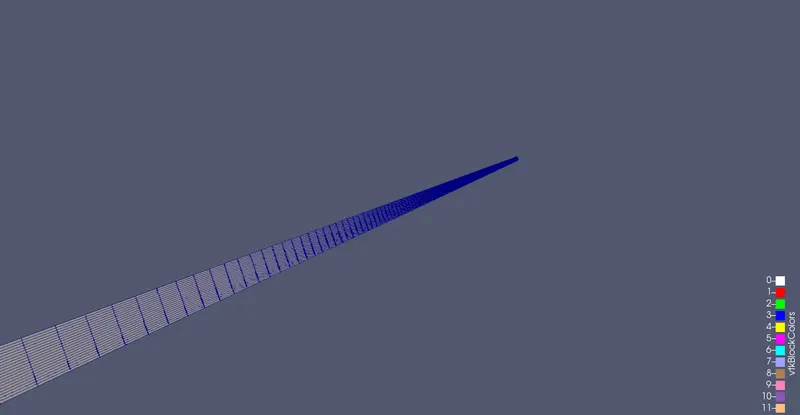
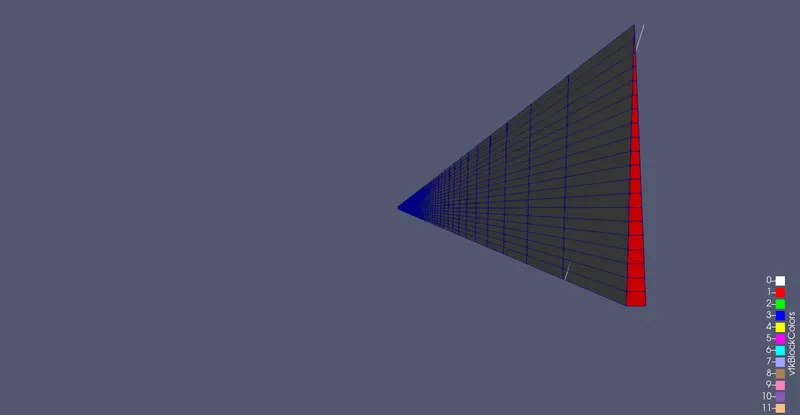
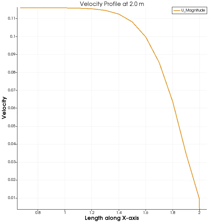
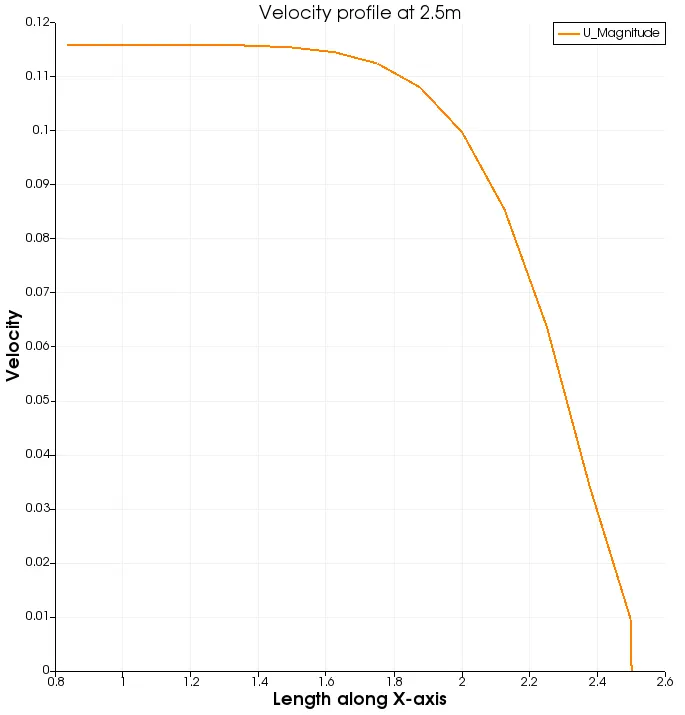
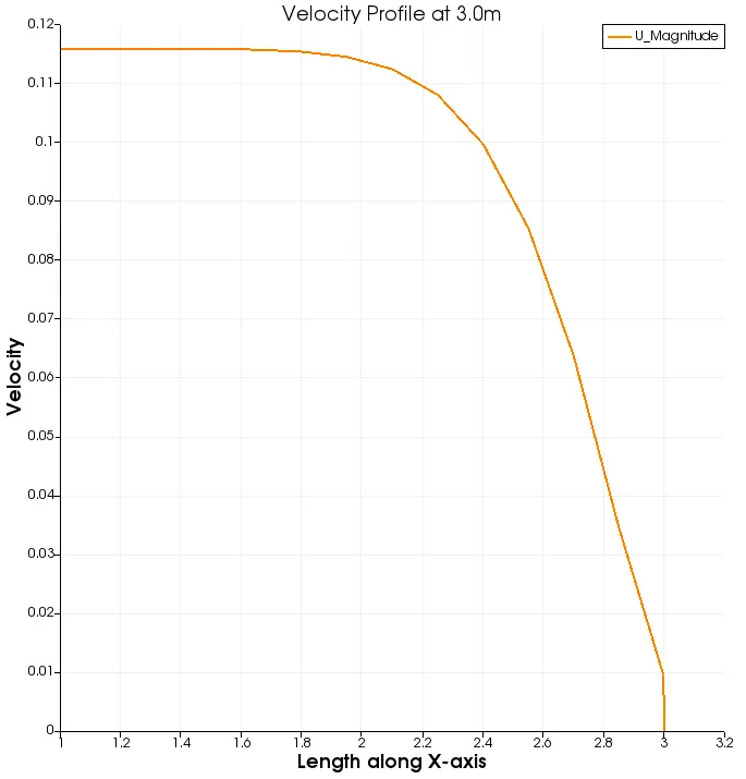
VELOCITY PROFILES AT DIFFERENT LENGHTS:

velocity profile at entry:

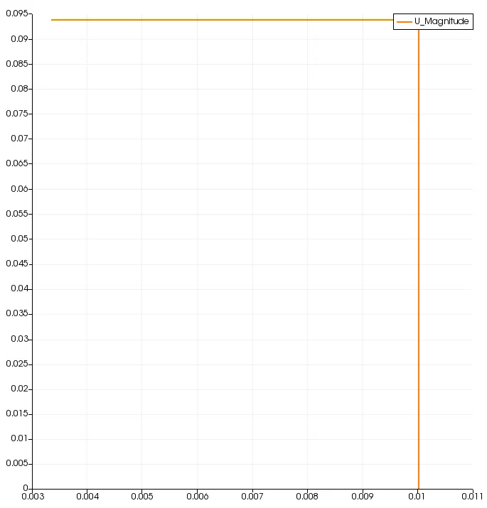
Velocity profile at length at 0.01m

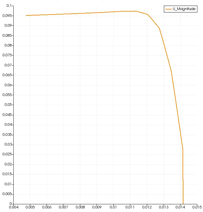
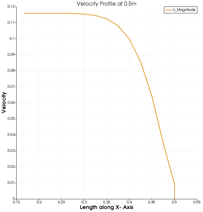
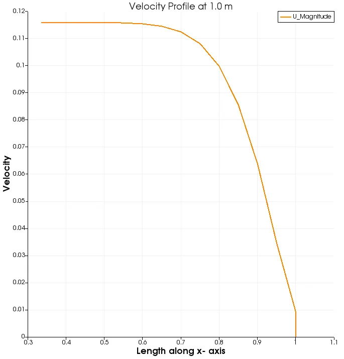
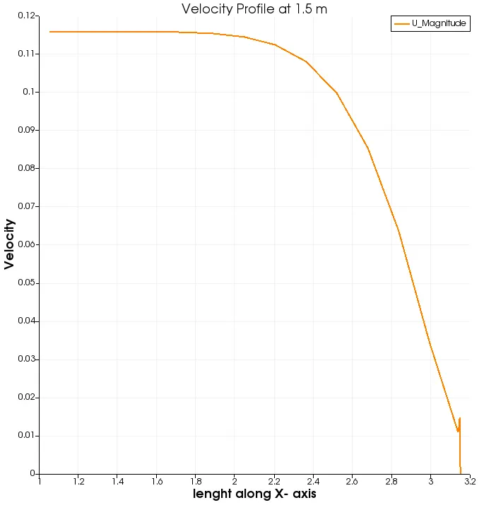
OBSERVATION:

From the above plots, it is evident that the plots of 2.5m and 3.0m are same, such that the flow is fully developed approximately after 2.5m and the length of total pipe assumed is under the limit. The plots are similar to the figure in introduction as at the entrance it is uniform initially and later drops at the end.

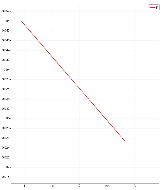
PRESSURE PROFILE ALONG THE LENGTH OF THE PIPE:

SHEAR STRESS IN FLUID FLOW:

A fluid at rest can not resist shearing forces. Under the action of such forces
it deforms continuously, however small they are. The resistance to the action of shearing forces in a fluid appears only when the fluid is in motion. This implies the principal difference between fluids and solids. For solids the resistance to a shear deformation depends on the deformation itself, that is the shear stress τ i s a function of the shear strain γ. For fluids the shear stress τ is a function of the rate of strain dγ/dt. The property of a fluid to resist the growth of shear deformation is called viscosity. The form of the relation between shear stress and rate of strain depends on a fluid, and most common fluids obey Newton’s law of viscosity, which states that the shear stress is proportional to the strain rate:

τ = µ*(du/dy)

CALUCULATING SHEAR STRESS ANALYTICALLY BY USING MATLAB:

clear all
close all
clc

%caluculating shear stress analytically
d = 0.02
r = d/2;
ra = linspace(0,0.005,500);
rho = 997;
mu = 0.00089;
Re = 2100;
u_avg = (Re*mu)/(rho*d);
u_max = 2*u_avg
  
for i = 1:length(ra)
  tau_a(i) = (2*mu*u_max*abs(ra(i)))/ (r^2)
endfor

figure(1)
plot(ra,tau_a)
xlabel('Radial Distance in m')
ylabel( 'Analytical Shear Stress in N/m^2')
legend( 'Shear stress plot along raduis')
grid on

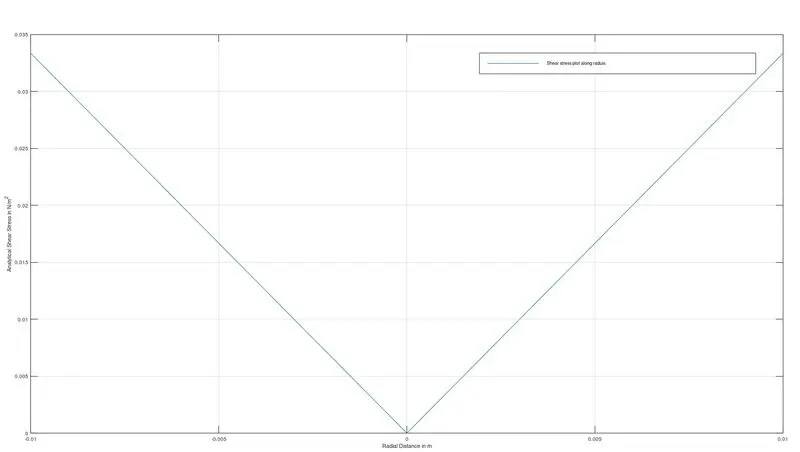
RESULTING PLOT FOR FULLY DEVELOPED FLOW:

CALUCULATING SHEAR STRESS NUMERICALLY USING PARAVIEW:

1) After sucessfully plotting the velocity priofiles, we will start to caluculate shear stress in paraview. Before starting we need to check the case ran upto last time step.

2) The next step is to open the caluculator by using tools> common> caluculator, in properties window we need to get the velocity magnitudes first by using vector option or else simply by typing mag(U) in formula bar and by giving the resuting array with a proper name as mag_U.

3) Then the array will apper in the field variable selection .

4) The next step is to to get the gradients of velocity magnitude along radius which is nothing but (du/dy). This can be done by using Gradientsofunstuctureddataset option. To access this option we have pess ctrl+space or in filters>search.

5) Then we will select the scalar array as mag_U and giving the resulting array with name as grad_mag_U and it will appear in variable selection window.

6) We know the formula for tau is mu*(du/dy), as we already got the gradients and the value for dyanamic viscosity of standard water as 0.00089 N/m^2.

7)To get this again we need open the caluculator, and in the formula bar, typing grad_mag_U*0.00089 and giving the resuting array with name of tau.

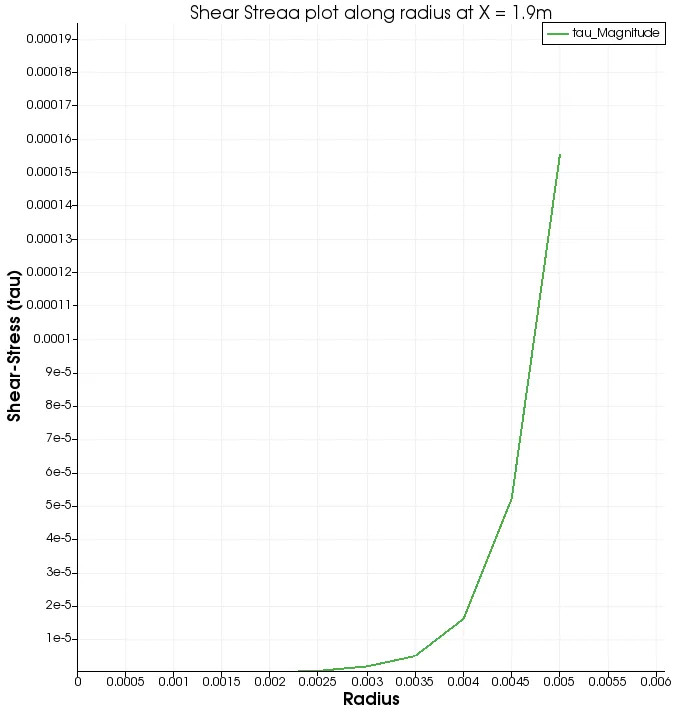
8) Then we can plot the shear stress profile by using plot over lime command and giving the axes with proper names.

OBSERVATIONS:

1) From velocity profiles, it is evident that at the entry the flow is uniform and after the hydrodynamic length of the pipe, the flow is fully developed. It can be seen that after the plots of 2.0m , the plots are very similar to each, this can tell us that the flow is fully developed around 1.9m.

2) From pressure plot, at the entry of the pipe, the pressure is very high and after flowing along the pipe it is coming down linearly. This is because of the shear stresses of the fluid.

3) From the Shear stress plot, we can observe that at the walls, the shear stress is very high and it is coming down to minimal at the centre of the pipe.