Week 9 - FVM Literature Review

The partial differential equations (PDEs) are of different nature, e.g. elliptic, parabolic, or hyperbolic, and are used as models in a wide number of fields and they describe the relations between partial derivatives of unknown fields such as temperature, concentration, pressure, the molar fraction with respect to variables within the domain (space, time,..etc) under consideration. These PDEs are discretized to form governing equations for various processes. Discretization is the process of converting PDE into Algebraic form.

Methods to discretize PDEs are

1. Finite Difference Method (FDM)
   • The finite-difference method is the most direct approach to discretizing partial differential equations. You consider a point in space where you take the continuum representation of the equations and replace it with a set of discrete equations, called finite-difference equations. The finite-difference method is typically defined on a regular grid and this fact can be used for very efficient solution methods.
2. Finite Element Method (FEM)
   • The finite-element method is a computational method that subdivides a CAD model into very small but finite-sized elements of geometrically simple shapes. The collection of all these simple shapes constitutes the so-called finite-element mesh.
3. Finite Volume Method (FVM)
   • The finite-volume method is similar to the finite-element method in that the CAD model is first divided into very small but finite-sized elements of geometrically simple shapes. The finite-volume method is based on the fact that many physical laws are conservation laws—what goes into one cell on one side needs to leave the same cell on another side.

Why the Finite Volume Method is used popularly?

FDM is used directly to a body whose grid points are not aligned properly along with x and y directions, these may occur due to complex flows, cuts in the structure. As it is not aligned we cannot calculate the properties at the next adjacent point exactly but we can make some correction factor and approximate it using "Variable transformation method" which basically seeks to create a grid using different variable space which looks very similar to a cartesian grid. But it is time consuming, complex, and thus is less preferred.

The finite volume method (FVM) is a method for representing and evaluating partial differential equations in the form of algebraic equations in the finite volume method volume integrals in a partial differential equation that contain a divergence term are converted to surface integral, using the divergence theorem These terms are then evaluated as fluxes at the surfaces of each finite volume. Because the flux entering a given volume is identical to that leaving the adjacent volume, these methods are conservative. Another advantage of the finite volume method is that it is easily formulated to allow for unstructured meshes. Finite volume refers to the small volume surrounding each node point on a mesh

In FVM instead of writing the equation in a single point, equations are written in an entire volume. It means for a considered volume no assumptions are made over the shape of the volume. Inside the particular volume, the flow is conserved flow quantities are conserved, energy is conserved, mass is conserved, momentum is conserved, and so on. This is called Finite Volume Representation which begins with an Integral form of governing equation

FVM computes solution at each finite volume whereas FDM computes solution at each point.

Steps in Finite Volume Method Discretization:

• Obtain the governing equation in its integral form
• Apply gauss divergence theorem
• Come up with a suitable method to calculate flux terms

consider a steady-state 1D heat conduction equation:

`del/(delx)(alpha.(delT)/(delx))+S=0`

`(delT)/(delx)`is temperature gradient along x-direction.

`alpha` is a thermal diffusivity term.

S is the source term.

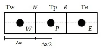
The governing equation above stated is valid at every point in the domain, therefore valid in the entire control volume.

Suppose a small control volume(dv) is considered and multiplied with the governing equation and integrating it for the entire control volume, which should also be equal to zero. taking the conservation equation validated at a single point then it is validated at the entire control volume and in this entire control volume properties are conserved.

`int (del/(delx)(alpha(delT)/(delx))+S)dv=0`

`int (del/(delx)(alpha(delT)/(delx)))dv+int(S)dv=0`

`dv=A.dx`

`int (del/(delx)(alpha(delT)/(delx)))A.dx+int(S)dv=0`

`[alpha.A((delT)/(delx))]_w^e+barSdv=0`

`barS`is the average value of source term (s) which when multiplied by dv is going to equal to `intSdv`

`alpha_e.A((delT)/(delx_e))-alpha_w.A((delT)/(delx_w))+barSdv=0`

we assume `alpha`as constant and not a function of temperature,

`alphaA[(T_e-T_p)/(Deltax)]-alphaA[(T_p-T_w)/(Deltax)]+barSdv=0`

the source term which is to be added in a cell, it is a function of temperature we have to linearize it.

`barS_(l i n erazation)to S_u+S_pT_p`

`alphaA[(T_e-T_p)/(Deltax)]-alphaA[(T_p-T_w)/(Deltax)]+(S_u+S_pT_p)dv=0`

`[Heat flux]_(out)-[Heat flux]_(i n)+Source term=0`

the amount of heat that is removed from a particular box is conserved.

The need for interpolation scheme in FVM:

The approximation of surface and volume integrals require values of the variable at a location other than computational nodes of the CV. Values at this location are obtained by an interpolation scheme.

Different interpolation scheme

1. Linear interpolation

• It is the simplest and most widely used interpolation. In this case, we can approximate the values of the control volume face center by interpolating the values linearly art the two nearest computational nodes.
• The linear interpolation is equivalent to the use of the central difference formula of the first-order derivative and hence it is also called as Central Difference Scheme(CDS). It is second-order accurate whose accuracy is very good but we might have one small problem for advection-dominated situations, that this scheme may produce oscillatory solutions. This scheme leads to a simple approximation for the evaluation of gradients required for the evaluation of diffusive fluxes.

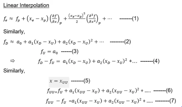
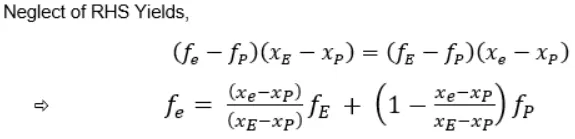
`lamda_e=`Function which would depend on the relative location of the computational nodes E and P w.r.t. eastern face

2. Upwind interpolation

• Here, we would require an upwind interpolation scheme which is essentially used for convection dominated problems, and here the velocity at a given point direction of that which determines the variable values to be used in the interpolation process, the name upwind refers to that we are going to make use of the node which is upwind or upstream of the given node,
• The upwind interpolation for approximating the value of a variable ‘f’ at the east face of the control volume is given as below. We want approximation at the eastern face ‘e’.

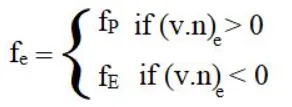
• `(v.n)_e`= is the velocity component at point e in the x-direction
• For the east face of a quantity, it is given as

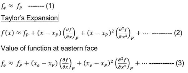
Comparison of UDS approximation with Taylor's series approximation clearly shows that the error in UDS approximation,

Let the epsilon be the error,

error in UDS approximation,

Where the second-order term is the leading truncation error which resembles a diffusive flux. UDS is the only approximation that satisfies the boundedness criterion unconditionally, in the sense that irrespective of what the velocity values are and irrespective of what is the grid spacing the solution will always remain bounded. It is first-order accurate in space.

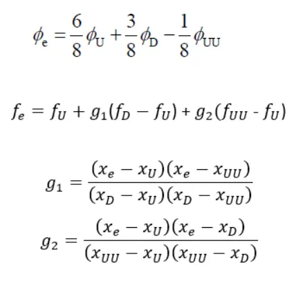
3. Quadratic upwind interpolation scheme

• In this case, we have to approximate the value of the variable at the Control Volume face center by quadratic interpolation of the values of the three nearest computational nodes.
• It is a third-order flux approximation, although it has a second-order overall accuracy.

4. Hybrid interpolation

• This scheme is the combination of upwind interpolation and a central differencing scheme based on the local Peclet number.
• `F_e=gamma F_(cds)+ (1-gamma)F_(cds)`

Flux limiters in FVM

High accurate and oscillation free scheme is known as High-resolution schemes.

They are used in higher resolution schemes, to avoid the false oscillation that would otherwise occur with a higher-order spatial discretization scheme due to shocks, discontinuities, or sharp changes in the solution domain. The main idea behind the construction of flux limiter schemes is to limit the spatial derivative to realistic values. They help to keep the values bounded at the cell faces. Thus they don’t let the solution value overshoot.

Consider the 1D semi-discrete scheme below,

`(du_i)/dt+1/(Deltax_i)[F(u_(i+1/2))-F(u_(i-1/2))]=0`

where `F(u_(i+1/2))` and `F(u_(i-1/2))` represents edge fluxes for the ith cell. If these edge fluxes can be represented by the low and high-resolution scheme, then a flux limiter can switch between these schemes depending upon the gradients close to the particular cell, as follows,

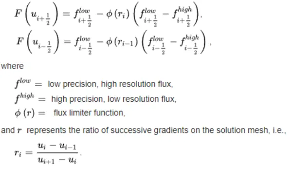
The limiter function is considered to be greater than or equal to zero i.e `phi(r_i)>=0`.

Therefore, when the limiter is equal to zero (sharp gradient, opposite slopes, or zero gradients), the flux is represented by a low-resolution scheme, similarly, when the limiter is equal to 1 (smooth solution), it is represented by a higher resolution scheme.