Week 7 - Simulation of a 1D Super-sonic nozzle flow simulation using Macormack Method
Aim:
To simulate the isentropic flow through a quasi 1D subsonic-supersonic nozzle using the Macormack method.
Introduction:
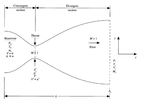
We consider a steady, isentropic flow through a convergent-divergent nozzle. This nozzle consists of a convergent section, throat section, and divergent section. The flow at the inlet to the nozzle comes from a reservoir where the pressure and temperature are denoted as `P_0` and `T_0` respectively. The cross-sectional area is large and hence velocity is very small. Here we are dealing with a particular case of Quasi 1D flow which means the flow is varied only in x-direction.
Mach number is a dimensionless quantity representing the ratio of flow of velocity to the local velocity of sound.
In the convergent section, this Mach number is less than 1 (M<1) therefore it is called Subsonic flow through the nozzle. In the divergent section, it is greater than 1 (M>1) thus called supersonic flow as the velocity of fluid-particle is more than that of sound. In the throat section velocity of the fluid-particle is equal to the local velocity of sound (M=1).
Governing Equation:
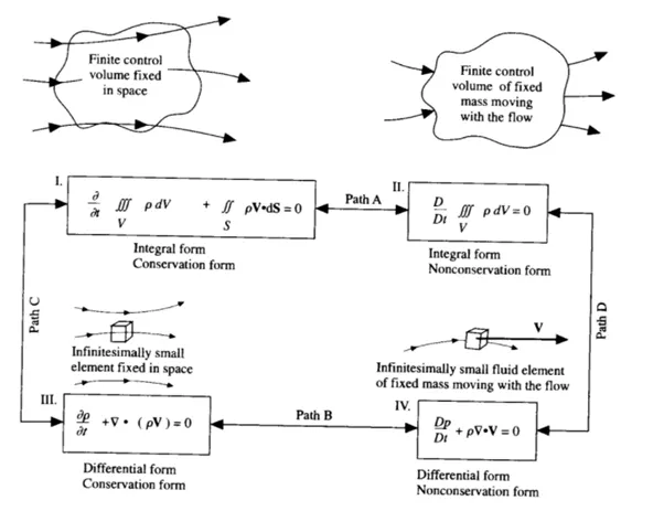
The flow through the nozzle is governed by the Navier Stokes equation which can be represented in both conservation and non-conservation form. Also, they can be further expressed in terms of integral and differential forms. All this equation can be converted into other just by doing mathematical operations on them.
To reduce the complexity of the notation we drop the use of prime to denote a dimensionless variable for density, temperature, velocity, and area.
Non conservation form:



Conservation form:
Continuity: 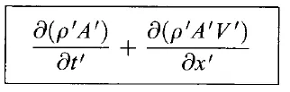 =0
=0
Momentum: 
Energy: 
where,
the dimensionless quantity is stated as
`T'=T/T_0`=`(Flow __temperature)/(Reserviour__temperature)`
`rho'=rho/rho_0`= `(Flow__density)/(Reserviour__ density)`
`x'=x/L` L is nozzle Length
`V'=V/a_0`=`(Flow __velocity)/(Speed__of__sound)`
`A'=A/A_0=( Area__of__nozzl e)/(Throat__area__at__sonic__section)`
Mac-Cormack method:
MacCormack's method is an explicit finite difference scheme for second-order accuracy with first-order terms in both space and time. It is a variant of the Lax-Wendroff approach but in a simpler way. Here, it uses the predictor-corrector step wherein the predictor step, space terms are replaced by forward differencing, and in the corrector step, they are replaced by backward differencing. The solution is updated and average time derivatives of predictor and corrector step are calculated for every grid point and time step.
Steps for Non-conservative form:
1) Setting up initial conditions
The area of the nozzle varies as

At x=1.5 is the throat of the nozzle, convergent section occurs for x<1.5, and the divergent section occurs at x>1.5
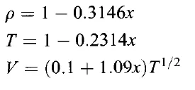
Initial conditions for density(rho), temperature(t) & velocity(v)
2) Calculation of the time step
Time step can be found by CFL criteria for 1D flow,
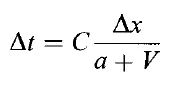
Where C=courant number, a= local speed of sound`=sqrtT`, V=local flow velocity at a point in the flow
Therefore, a new time step will be
`Deltat=min( C. (Deltax)/(sqrtT'+V'))`
These time steps are calculated for all given temperature and velocity grid points and then the minimum of it is considered.
3) Predictor step
We set up spatial derivatives as forwarding differences.
For the continuity equation,

For the Momentum equation,

For the energy equation,

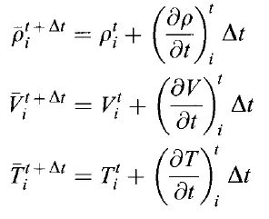
Now we obtain predicted quantity using the Taylor series,
4) Corrector step
Here we set up spatial derivatives as backward differences.
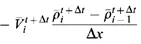
For the continuity equation,

For the momentum equation,

For the energy equation,


The average timer derivative is calculated both from the predictor and corrector step.
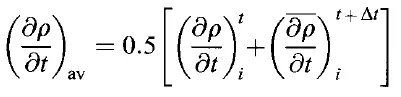
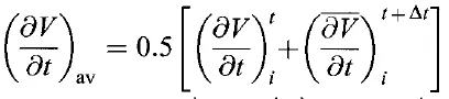
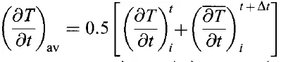
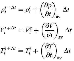
The final solution will be,
5) Boundary conditions (B.C)
These are important because, without the proper physical implementation and representation of boundary conditions, we may not obtain the proper solution for our flow problem. There will be 2 boundary conditions, one at point 1 in the grid representing inflow B.C (subsonic) and other at point N in the grid representing outflow B.C (supersonic).
Subsonic inflow B.C
We must stipulate the value of two independent flow variables whereas the value of one other variable must be allowed to float. We choose velocity (V) as float variable because on a physical basis we know the mass flow through the nozzle must be allowed to adjust to the proper steady state, thus allowing V to float makes sense as part of this adjustment.
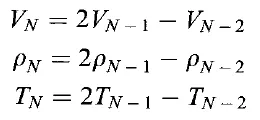
`V_1=2*V_2-V_3`
Supersonic outflow B.C
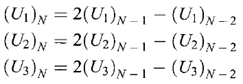
Here all the variables must be allowed to float. For this, we choose linear extrapolation based on the flow field variables at the internal points.
Steps for Conservative form:
1) Setting up initial conditions
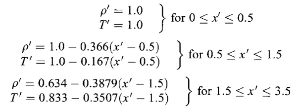
Values of density, temperature varies accordingly,
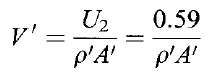
Value of mass flow
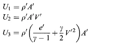
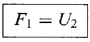
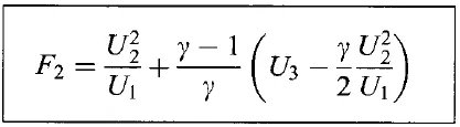
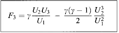
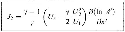
Here we have the solution vector U, Flux vector F, and the source term J as
A pure form of flux terms,
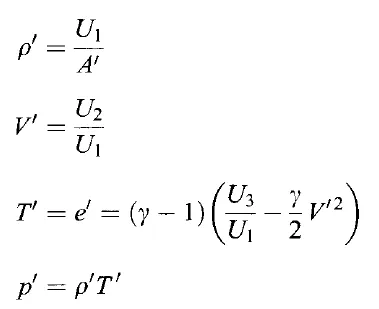
Primitive variables can be obtained using the solution vector by:
2) Calculation of the time step
"Same as non-conservation form"
3) Predictor step
Here Flux terms use a forward differencing scheme.
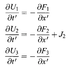
Then the solution is updated using the Taylor series
`barU_1^(t+Deltat)=U_1^t+((delU_1)/(delt))^t*Deltat`
Similarly for `bar(U_2)` and `bar(U_3)`
4) Corrector step
Here Flux terms are solved in backward differencing.
Then the average of predictor and corrector step is found the same as we did in non-conservative form.
At last, the final corrected step can be obtained by using the Taylor series.
Finally, the primitive variables are decoded by,
5) Boundary condition.
Subsonic inflow boundary flow
Two properties are fixed, one is allowed to float.
`U1(1)=rho(1)*a(1)`
`U2(1)=2*U2(2)-U2(3)`
`U3(1)=U1(1)*(((T(1))/(gamma-1))+(gamma/2)*V(1)^2)`
`V(1)=(U2(1))/(U1(1))`
Supersonic outflow boundary outflow
All properties are allowed to float.
MATLAB code:
Main code
clear all
close all
clc

%inputs
n=31;
L=3;
x=linspace(0,L,n);

%courrant number
c=0.5;

%time step
nt=1400;

tic
%function for non conservative form
[rho1,t1,v1,m1,mach1,pr1,rho_t1,t_t1,v_t1,m_t1,mach_t1,pr_t1]=non_conservative_flow(n,L,c,nt);
%simulation time(non conservative form)
non_cons_time=toc

tic
%function for conservative form
[rho2,t2,v2,m2,mach2,pr2,rho_t2,t_t2,v_t2,m_t2,mach_t2,pr_t2]=conservative_flow(n,L,c,nt);
%simulation time(conservative form)
cons_time=toc


%Variation of flow parameters along xaxis
figure(3)
subplot(4,1,1)
plot(x,rho1,'r','linewidth',1.5);
hold on
plot(x,rho2,'b*');
title('Variation of flow parameters along x axis')
ylabel("rho'")
legend('Non-conservation form','Conservation form')
set(legend,'location','northeastoutside')
grid on

subplot(4,1,2)
plot(x,pr1,'color','r','linewidth',1.5);
hold on
plot(x,pr2,'b*');
ylabel("pr'")
legend('Non-conservation form','Conservation form')
set(legend,'location','northeastoutside')
grid on

subplot(4,1,3)
plot(x,t1,'r','linewidth',1.5);
hold on
plot(x,t2,'b*');
ylabel("t'")
legend('Non-conservation form','Conservation form')
set(legend,'location','northeastoutside')
grid on

subplot(4,1,4)
plot(x,mach1,'r','linewidth',1.5);
hold on
plot(x,mach2,'b*');
ylabel("mach'")
legend('Non-conservation form','Conservation form')
set(legend,'location','northeastoutside')
grid on


%Variation of flow parameters at the throat(density, pressure,
%temperature,mach number)
figure(4)
subplot(4,1,1)
plot(linspace(1,nt,nt),rho_t1,'r','linewidth',1.5);
hold on
plot(linspace(1,nt,nt),rho_t2,'b','linewidth',1.5);
title('Variation of flow parameters')
ylabel("rho'")
legend('Non-conservation form','Conservation form')
set(legend,'location','northeastoutside')
grid on

subplot(4,1,2)
plot(linspace(1,nt,nt),pr_t1,'r','linewidth',1.5);
hold on
plot(linspace(1,nt,nt),pr_t2,'b','linewidth',1.5);
ylabel("pr'")
legend('Non-conservation form','Conservation form')
set(legend,'location','northeastoutside')
grid on

subplot(4,1,3)
plot(linspace(1,nt,nt),t_t1,'r','linewidth',1.5);
hold on
plot(linspace(1,nt,nt),t_t2,'b','linewidth',1.5);
ylabel("t'")
legend('Non-conservation form','Conservation form')
set(legend,'location','northeastoutside')
grid on

subplot(4,1,4)
plot(linspace(1,nt,nt),mach_t1,'r','linewidth',1.5);
hold on
plot(linspace(1,nt,nt),mach_t2,'b','linewidth',1.5);
ylabel("pr'")
legend('Non-conservation form','Conservation form')
set(legend,'location','northeastoutside')
grid on

%Mass flow rate comparison
figure(5)
plot(x,m1,'r','linewidth',1.5)
hold on
plot(x,m2,'b','linewidth',1.5)
xlabel('Mass flow rate')
ylabel('Distance through nozzle(x)')
title('Comparison of mass flow rate')
legend('Non-conservation form','Conservation form')
Function Code:
Non-conservative form:
function [rho1,t1,v1,m1,mach1,pr1,rho_t1,t_t1,v_t1,m_t1,mach_t1,pr_t1]=non_conservative_flow(n,L,c,nt)

%inputs
x=linspace(0,L,n);
dx=x(2)-x(1);
gamma=1.4;

%area of nozzle
a=1+2.2*(x-1.5).^2;
%area at throat
throat=find(a==1)

%calculate initial profile
rho1= 1-0.3146*x;
t1=1-0.2314*x;   %t=temperature
v1=(0.1+1.09*x).*t1.^0.5;

for i=1:n
  dt_cal(i)= (c*dx)/((t1(i)).^0.5+v1(i));
end
dt=min(dt_cal);

%outer time loop
for k=1:nt

    rho_old=rho1;
    t_old=t1;
    v_old=v1;

    %predictor step
    for j = 2:n-1

        dvdx=(v1(j+1)-v1(j))/dx;
        drhodx=(rho1(j+1)-rho1(j))/dx;
        dtdx=(t1(j+1)-t1(j))/dx;
        dlogadx=(log(a(j+1))-log(a(j)))/dx;

        %continunty equation
        drhodt_p(j)=-rho1(j)*dvdx-rho1(j)*v1(j)*dlogadx-v1(j)*drhodx;

        %momentum equation
        dvdt_p(j)=-v1(j)*dvdx-(1/gamma)*(dtdx+(t1(j)/rho1(j))*drhodx);

        %energy equation
        dtdt_p(j)=-v1(j)*dtdx-(gamma-1)*t1(j)*(dvdx+v1(j)*dlogadx);

        %solution update
        v1(j) = v1(j) + dvdt_p(j)*dt;
        t1(j) = t1(j) + dtdt_p(j)*dt;
        rho1(j) = rho1(j) + drhodt_p(j)*dt;

    end

    %corrector step
    for j = 2:n-1

        dvdx=(v1(j)-v1(j-1))/dx;
        drhodx=(rho1(j)-rho1(j-1))/dx;
        dtdx=(t1(j)-t1(j-1))/dx;
        dlogadx=(log(a(j))-log(a(j-1)))/dx;

        %continunty equation
        drhodt_c(j)=-rho1(j)*dvdx-rho1(j)*v1(j)*dlogadx-v1(j)*drhodx;

        %momentum equation
        dvdt_c(j)=-v1(j)*dvdx-(1/gamma)*(dtdx+(t1(j)/rho1(j))*drhodx);

        %energy equation
        dtdt_c(j)=-v1(j)*dtdx-(gamma-1)*t1(j)*(dvdx+v1(j)*dlogadx);

    end

    %compute the avg time value
    drhodt=0.5*(drhodt_p + drhodt_c);
    dvdt=0.5*(dvdt_p + dvdt_c);
    dtdt=0.5*(dtdt_p + dtdt_c);

    for i=2:n-1
    %Final solution
    rho1(i) = rho_old(i) + drhodt(i)*dt;
    v1(i) = v_old(i) + dvdt(i)*dt;
    t1(i) = t_old(i) + dtdt(i)*dt;
    end

    %apply the boundary conditions
    %inlet
    v1(1)=2*v1(2)-v1(3);

    %outlet
    rho1(n)=2*rho1(n-1)-rho1(n-2);
    v1(n)=2*v1(n-1)-v1(n-2);
    t1(n)=2*t1(n-1)-t1(n-2);

    %calculating solutions
    %mass flow rate
    m1=rho1.*v1.*a;
    %mach number
    mach1=v1./(t1.^0.5);
    %pressure ratio
    pr1=rho1.*t1;

    %throat values
    rho_t1(k)=rho1(throat);
    t_t1(k)=t1(throat);
    v_t1(k)=v1(throat);
    m_t1(k)=m1(throat);
    mach_t1(k)=mach1(throat);
    pr_t1(k)=pr1(throat);

    %plotting mass flow rate at different time steps
    figure(1)
    if k==50
        plot(x,m1,'r','linewidth',1.5)
        hold on
    elseif k==100
        plot(x,m1,'b','linewidth',1.5)
        hold on
    elseif k==150
        plot(x,m1,'g','linewidth',1.5)
        hold on
    elseif k==200
        plot(x,m1,'y','linewidth',1.5)
        hold on
    elseif k==400
        plot(x,m1,'k','linewidth',1.5)
        hold on
    elseif k==800
        plot(x,m1,'c','linewidth',1.5)
        hold on
    elseif k==1400
        plot(x,m1,'m','linewidth',1.5)
        hold on
       grid on
       title('Variation of mass flow rate at different time step (Non-conservstive form)')
       ylabel('Non dimensional mass flow rate')
       xlabel('Length of nozzle')
       legend({'50 time steps','100 time steps','150 time steps','200 time steps','400 time steps','800 time steps','1400 time steps'});
    end
end
end
Conservative form:
function [rho,t,v,m,mach,pr,rho_t2,t_t2,v_t2,m_t2,mach_t2,pr_t2]=conservative_flow(n,L,c,nt)

%inputs
x=linspace(0,L,n);
dx=x(2)-x(1);
gamma=1.4;

%calculate initial profile
%area of nozzle
a=1+2.2*(x-1.5).^2;
%area at throat
throat=find(a==1);

%rho(density) and t (temperature)
for i=1:n
    if (x(i)>=0 && x(i)<=0.5)
        rho(i)=1;
        t(i)=1;
    elseif (x(i)>=0.5 && x(i)<=1.5)
        rho(i)=1-0.366*(x(i)-0.5);
        t(i)=1-0.167*(x(i)-0.5);
    elseif (x(i)>=1.5 && x(i)<=3.5)
        rho(i)=0.634-0.3879*(x(i)-1.5);
        t(i)=0.833-0.3507*(x(i)-1.5);
    end
end

%velocity
v=0.59./(rho.*a);

%solution vector
u1=rho.*a;
u2=rho.*a.*v;
u3=rho.*a.*((t./(gamma-1))+((gamma/2).*(v.^2)));

%time step
dt=min((c.*dx)./(t.^0.5+v));

%outer time loop
for k=1:nt

    %copy terms
    rho_old=rho;
    t_old=t;
    v_old=v;

    u1_old=u1;
    u2_old=u2;
    u3_old=u3;

    %flux terms
    f1=u2;
    f2=((u2.^2)./u1)+(((gamma-1)/gamma).*(u3-((gamma/2)*((u2.^2)./u1))));
    f3=(((gamma.*u2.*u3)./u1)-((gamma*(gamma-1)/2).*(u2.^3./u1.^2)));

    %predictor step
    for j = 2:n-1

        df1dx(j)=(f1(j+1)-f1(j))/dx;
        df2dx(j)=(f2(j+1)-f2(j))/dx;
        df3dx(j)=(f3(j+1)-f3(j))/dx;

        dadx(j)=(a(j+1)-a(j))/dx;
        j2(j)=(1/gamma)*(rho(j)*t(j))*dadx(j);

        %continunty equation
        du1dt_p(j)=-df1dx(j);

        %momentum equation
        du2dt_p(j)=-df2dx(j)+j2(j);

        %energy equation
        du3dt_p(j)=-df3dx(j);

        %solution update
        u1(j)=u1(j)+du1dt_p(j)*dt;
        u2(j)=u2(j)+du2dt_p(j)*dt;
        u3(j)=u3(j)+du3dt_p(j)*dt;

    end

    %obtainig primitive variables and flux value
    rho=u1./a;
    v=u2./u1;
    t=(gamma-1)*((u3./u1)-((gamma*(v.^2))./2));

    f1=u2;
    f2=((u2.^2./u1)+(((gamma-1)/gamma).*(u3-(gamma/2)*(u2.^2./u1))));
    f3=(((gamma.*u2.*u3)./u1)-((gamma*(gamma-1)/2).*(u2.^3./u1.^2)));

    %corrector step
    for j = 2:n-1

        df1dx(j)=(f1(j)-f1(j-1))/dx;
        df2dx(j)=(f2(j)-f2(j-1))/dx;
        df3dx(j)=(f3(j)-f3(j-1))/dx;

        dadx1(j)=(a(j)-a(j-1))/dx;
        j3(j)=(1/gamma)*(rho(j)*t(j))*dadx1(j);

        %continunty equation
        du1dt_c(j)=-df1dx(j);

        %momentum equation
        du2dt_c(j)=-df2dx(j)+j3(j);

        %energy equation
        du3dt_c(j)=-df3dx(j);

    end

    %compute the avg time value
    du1dt=0.5*(du1dt_p + du1dt_c);
    du2dt=0.5*(du2dt_p + du2dt_c);
    du3dt=0.5*(du3dt_p + du3dt_c);

    for i=2:n-1
    %Final solution
    u1(i)=u1_old(i)+du1dt(i)*dt;
    u2(i)=u2_old(i)+du2dt(i)*dt;
    u3(i)=u3_old(i)+du3dt(i)*dt;
    end

    %apply the boundary conditions
    %inlet
    u1(1)=rho(1)*a(1);
    u2(1)=2*u2(2)-u2(3);
    v(1)=u2(1)/u1(1);
    u3(1)=u1(1)*((t(1)/(gamma-1))+((gamma/2)*v(1)^2));

    %outlet
    u1(n)=2*u1(n-1) - u1(n-2);
    u2(n)=2*u2(n-1) - u2(n-2);
    u3(n)=2*u3(n-1) - u3(n-2);

    %final values of primtive variables
    rho=u1./a;
    v=u2./u1;
    t=(gamma-1)*((u3./u1)-((gamma/2)*(v.^2)));

    %calculating solutions
    %mass flow rate
    m=rho.*v.*a;
    %mach number
    mach=v./(t.^0.5);
    %pressure ratio
    pr=rho.*t;

    %throat values
    rho_t2(k)=rho(throat);
    t_t2(k)=t(throat);
    v_t2(k)=v(throat);
    m_t2(k)=m(throat);
    mach_t2(k)=mach(throat);
    pr_t2(k)=pr(throat);

    %plotting mass flow rate at different time steps
    figure(2)
    if k==50
        plot(x,m,'r','linewidth',1.5)
        hold on
    elseif k==100
        plot(x,m,'b','linewidth',1.5)
        hold on
    elseif k==150
        plot(x,m,'g','linewidth',1.5)
        hold on
    elseif k==200
        plot(x,m,'y','linewidth',1.5)
        hold on
    elseif k==400
        plot(x,m,'k','linewidth',1.5)
        hold on
    elseif k==800
        plot(x,m,'c','linewidth',1.5)
        hold on
    elseif k==1400
        plot(x,m,'m','linewidth',1.5)
        hold on
       grid on
       title('Variation of mass flow rate at different time step (conservative form)')
       ylabel('Non dimensional mass flow rate')
       xlabel('Length of nozzle')
       legend({'50 time steps','100 time steps','150 time steps','200 time steps','400 time steps','800 time steps','1400 time steps'});
    end
end
end
Output & Conclusion:
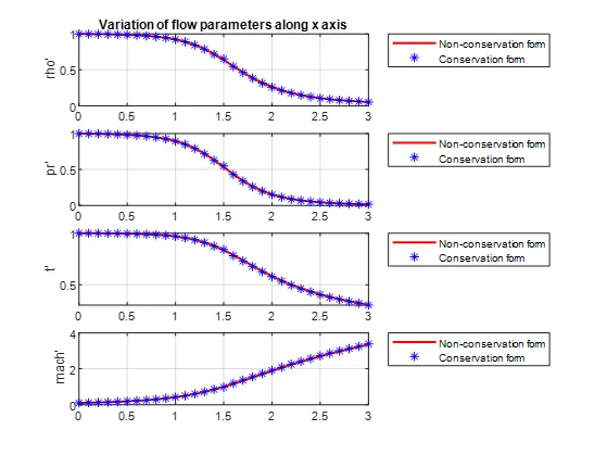
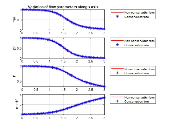
1) Steady-state distribution of primitive variables inside the nozzle
From the graph, it can be inferred that the conservation form is more stable than compared to non-conservation form as the variation is less. It can also be inferred that after 400-time steps the graph stabilizes and proceeds almost linearly.
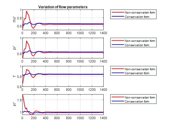
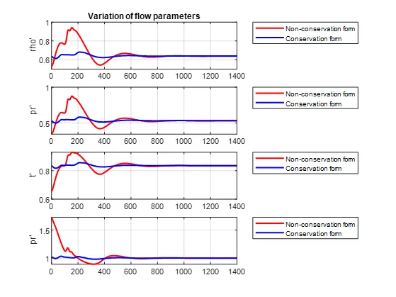
2) Time-wise variation of the primitive variables
A similar result can be obtained for both conservation and non-conservation form in terms of primitive variables(Density, Pressure ratio, Temperature, Mach No.) at the throat section. Thus we can conclude that both governing equations conclude the same results for this flow problem through the nozzle. But when the shock wave is considered the results will deviate for both conservational and non-conservational forms.
3) Variation of Mass flow rate distribution inside the nozzle at different time steps during the time-marching process
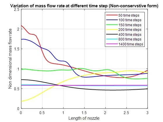
Non-conservative form:
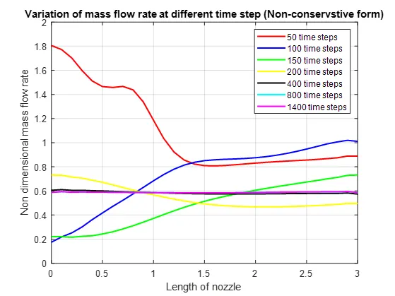
It can be seen from the graph that after a 400-time step the graph stabilizes and negligible change can be seen for a later time step.
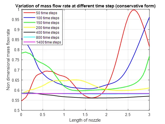
Conservative form:
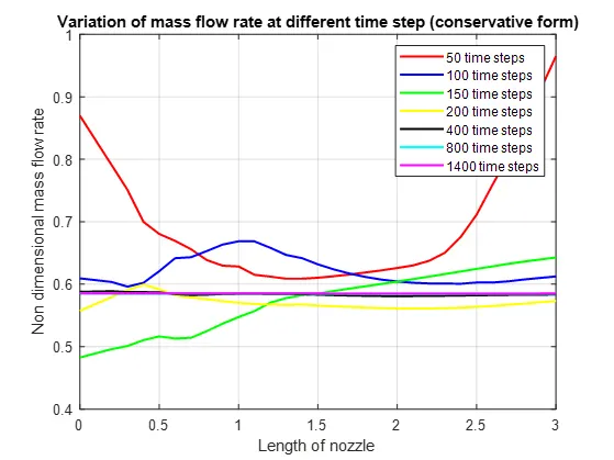
It can be inferred that the graph starts stabilizing after 400-time steps. Since then very less change can be seen.
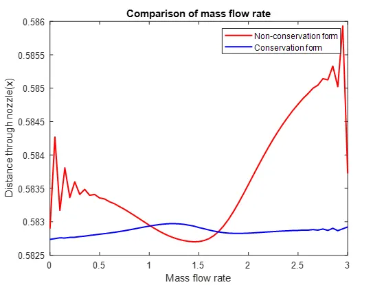
4) Comparison of Normalized mass flow rate distributions of both forms
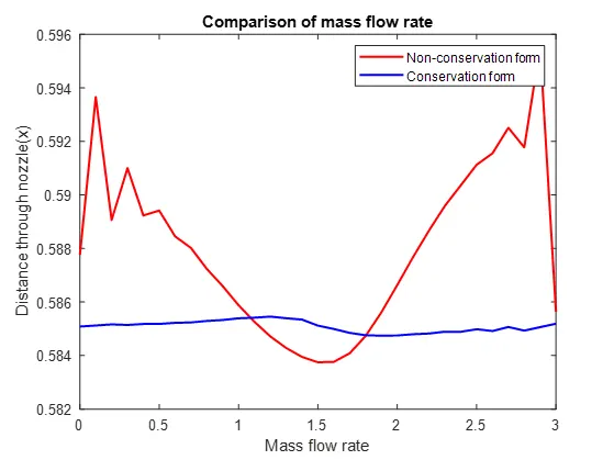
From the plot, we can see that the mass flow rate for the non-conservation form varies a lot when compared to the conservation form which appears to be stable. Also, the conservation form is close to the analytical solution as given in the book.
5) Grid Dependency test
| rho' | T' | P' | Mach no. | |
| Exact analytical solution | 0.634 | 0.833 | 0.528 | 1 |
| Non-Conservational form (Grid size=31) | 0.6387 | 0.8365 | 0.5342 | 0.9994 |
| Conservational form (Grid size=31) | 0.6534 | 0.8410 | 0.5487 | 0.9780 |
| Non- Conservational form (Grid size=61) | 0.6377 | 0.8354 | 0.5327 | 0.9998 |
| Conservational form (Grid Size=61) | 0.6391 | 0.8355 | 0.5340 | 0.9979 |
Thus we can conclude that after 31 grid size if we increases its refinement it will result in similar results and no major change will be obtained for primitive values. the results of non-conservation form are more close to analytical solution than that of conservation form.
6) Effect of CFL number (Non-Conservation form)
| Courant number | rho' | T' | P' | Mach no. |
| Exact analytical solution | 0.634 | 0.833 | 0.534 | 1 |
| 0.5 | 0.6387 | 0.8365 | 0.5342 | 0.9994 |
| 0.7 | 0.6391 | 0.8366 | 0.5346 | 0.9992 |
| 0.9 | 0.6395 | 0.8368 | 0.5351 | 0.9989 |
| 1.1 | 0.6399 | 0.8369 | 0.5355 | 0.9987 |
| 1.2 | NaN | NaN | NaN | NaN |
we get get accurate results till c=1.1 after that the solution is blown away.
7) Computational time
| Time(s) | |
| Non-Conservation form (Grid size=31) | 3.6871 |
| Conservation form (Grid size=31) | 3.8336 |
| Non-Conservation form (Grid size=61) | 3.5711 |
| Conservation form (Grid size=61) | 3.9001 |
The time conservation is little more than a non-conservation form that may be due to little more complexity in solving the equations
Appendix:
Figures for grid size=61
1. Steady-state distribution of primitive variables inside the nozzle
2. Time-wise variation of the primitive variables
3. Variation of Mass flow rate distribution inside the nozzle at different time steps during the time-marching process
4. Comparison of Normalized mass flow rate distributions of both forms