Week 5 - Mid term project - Solving the steady and unsteady 2D heat conduction problem

AIM:

To solve the steady and unsteady 2D heat conduction Problem

THEORY:

Steady-State 2D Heat Conduction

The generalized 2D steady-state heat conduction equation with no heat generation equation is given as

`(del^2T)/(delx^2)+(del^2T)/(dely^2)=0`...................(1)

this equation is discretized by central difference scheme for x and y directions

`(del^2T)/(delx^2)=(T_(i-1,j)-2T_(i,j)+T_(i+1,j))/(Deltax^2)`....................(2)

`(del^2T)/(dely^2)=(T_(i,j-1)-2T_(i,j)+T_(i,j+1))/(Deltay^2)`....................(3)

therefore placing this in equation 1, we get

`(T_(i-1,j)-2T_(i,j)+T_(i+1,j))/(Deltax^2)+(T_(i,j-1)-2T_(i,j)+T_(i,j+1))/(Deltay^2)=0`...............(4)

further, for this problem, we are putting `Deltax=Deltay`...........(5)

therefore placing equation 5 in 4, we get

`T_(i,j)=1/4(T_(i-1,j)+T_(i+1,j)+T_(i,j-1)+T_(i,j+1))`

As we solve this equation for a very time loop we get error i.e previous temperature - new temperature. the solution stabilizes only when this error falls below the tolerance limit which is 1e-4 for the current problem. So the heat conduction equation has to be solved using iterative steps for the implicit scheme. There are 3 iterative types available to solve this problem:

1) Jacobi Method

Here all the values in RHS are taken from previous time step

`T_(i,j)^(n+1)=1/4(T_(i-1,j)^n+T_(i+1,j)^n+T_(i,j-1)^n+T_(i,j+1)^n)`

2) Gauss-Seidal Method

Here the new values of T from space loop are used wherever its possible in next time loop. thus reduces number of iteration than jacobi

`T_(i,j)^(n+1)=1/4(T_(i-1,j)^(n+1)+T_(i+1,j)^n+T_(i,j-1)^(n+1)+T_(i,j+1)^n)`

3) Successive Over Relaxtion Method

Here the solution of gauss-sedal is further multiplied by over relaxation factor (`omega`). This `omega` lies between 1 and 2 so that we can stablize the solution quickly then the later.

`T_(i,j)^(n+1)=(1-omega)T_(i,j)^(n)+omega(T_(i,j)(gs))`

where `T_(i,j)(gs)` is the solution obtained from gauss seidal method.

MATLAB CODE:

Select the iterative solver as per the need (1,2,3)

%solving 2D heat conduction equation
%d^2t/dx^2+d^2t/dy^2=0

clear all
close all
clc

%inputs
nx=10;
ny=10;
x=linspace(0,1,nx);
y=linspace(0,1,ny);
dx=x(2)-x(1);
dy=y(2)-y(1);
[X,Y]=meshgrid(x,y)
tol=1e-4;
error=9e9;

T=zeros(nx,ny);
omega=1.5;  %For SOR

%Assigning BC
T(:,1)=400; %left BC
T(:,nx)=800; %right BC
T(1,:)=600; %top BC
T(ny,:)=900; %bottom BC
%corner points
T(1,1)=500;
T(nx,1)=650;
T(1,ny)=700;
T(nx,ny)=850;

%creating a copy of T
Told=T;

%decide to go for jacobi or GS or SOR (1 or 2 or 3) 
iterative_solver=1;

%jacobi method
%as dx=dy therefore K=4
tic
    if iterative_solver==1
        jacobi_iter=1;
        
        while(error > tol)
            for i=2:nx-1
                for j=2:ny-1
                    T(i,j)=(1/4)*(Told(i-1,j)+Told(i+1,j)+Told(i,j-1)+Told(i,j+1));
                end
            end
        error= max(max(abs(Told-T)));
        Told=T;
        jacobi_iter=jacobi_iter+1;
        end
        F=toc;
        figure(1)
contourf(x,y,T);
[a,b]=contourf(x,y,T);
clabel(a,b);
ax=gca;
xlabel('X')
ylabel('Y')
colorbar
colormap(jet)
set(gca,'Ydir','reverse')
title_text=sprintf('No of Jacobi iteration=%d,\n Computational Time=%0.5f',jacobi_iter,F);
title(title_text)
    end

%gauss sedal method
%as dx=dy therefore K=4
 tic
 if iterative_solver==2
     gs_iter=1;
        while(error > tol)
            for i=2:nx-1
                for j=2:ny-1
                    T(i,j)=(1/4)*(T(i-1,j)+Told(i+1,j)+T(i,j-1)+Told(i,j+1));
                end
            end
        error= max(max(abs(Told-T)));
        Told=T;
        gs_iter=gs_iter+1;
        end
        F=toc;
        figure(2)
contourf(x,y,T);
[a,b]=contourf(x,y,T);
clabel(a,b);
xlabel('X')
ylabel('Y')
colorbar
colormap(jet)
set(gca,'YDIR','reverse')
title_text=sprintf('No of gauss-sedal iteration=%d, \n Computational Time=%0.5f',gs_iter,F);
title(title_text)
 end
 
%successive over relaxive method
%as dx=dy therefore K=4
 tic
 if iterative_solver==3
     sor_iter=1;
        while(error > tol)
            for i=2:nx-1
                for j=2:ny-1
                    T(i,j)=((1-omega)*Told(i,j))+omega*((1/4)*(T(i-1,j)+Told(i+1,j)+T(i,j-1)+Told(i,j+1)));
                end
            end
        error= max(max(abs(Told-T)));
        Told=T;
        sor_iter=sor_iter+1;
        end
        F=toc;
        figure(3)
contourf(x,y,T);
[a,b]=contourf(x,y,T);
clabel(a,b);
xlabel('X')
ylabel('Y')
colorbar
colormap(jet)
set(gca,'YDIR','reverse')
title_text=sprintf('No of SOR iteration=%d, \n Computational Time=%0.5f',sor_iter,F);
title(title_text)
    end
    

OUTPUT:

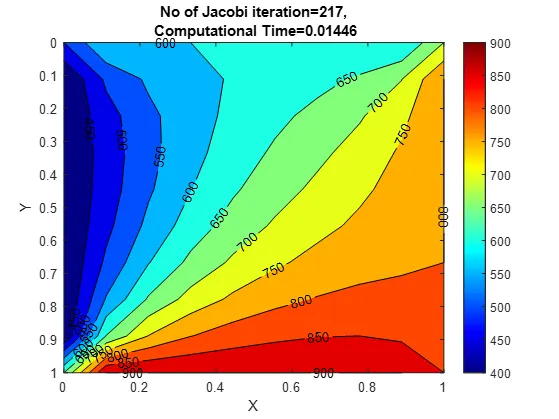
1) Jacobi

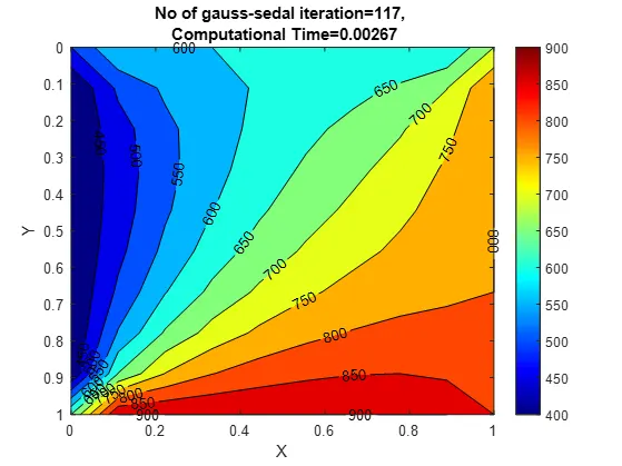
2) Gauss-Seidal

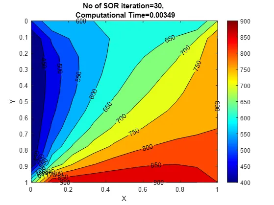
3) SOR

CONCLUSION:

Based on number of iteration : Jacobi > Gauss-seidel > SOR

Thus SOR method gives stable solution in very less iterations, but we should note that increasing omega value will start to oscillate the solution and furthermore say omega=2 will blow away the solution.

2D Unsteady state Heat conduction equation:

`(delT)/(delt)=alpha((del^2T)/(delx^2)+(del^2T)/(dely^2))`

the above equation can be solved in 2 ways -implicitcally and explicitically

1)Explicit method

discretizing it we get

`(T_(i,j)^(n+1)-T_(i,j)^n)/(Deltat)=alpha((T_(i-1,j)^n-2T_(i,j)^n+T_(i+1,j)^n)/(Deltax^2)+(T_(i,j-1)^n-2T_(i,j)^n+T_(i,j+1)^n)/(Deltay^2))`

Here if we bring all constant term towards RHS, a new term can replace all this constants. This new constant is called as CFL (Courant-Friedrich-Lewy) number that describes the stability of the equation.

`K1=alpha*(Deltat)/(Deltax^2)`

`K2=alpha*(Deltat)/(Deltay^2)`

Replacing constants,

as `Deltax=Deltay` for this current problem we can say that

K=K1=K2

therefore we get,

`T_(i,j)^(n+1)=T_(i,j)^n+K*(T_(i-1,j)^n+T_(i+1,j)^n+T_(i,j-1)^n+T_(i,j+1)^n-4T_(i,j)^n)`

`T_(i,j)^(n+1)=(1-4K)T_(i,j)^n+K*(T_(i-1,j)^n+T_(i+1,j)^n+T_(i,j-1)^n+T_(i,j+1)^n)`

MATLAB CODE:

close all
clear all
clc
%solving 2D heat conduction equation explicit
%delT/delt=alpha(d^2t/dx^2+d^2t/dy^2)

%inputs
nx=10;
ny=10;
x=linspace(0,1,nx);
y=linspace(0,1,ny);
dx=x(2)-x(1);
dy=y(2)-y(1);
[X,Y]=meshgrid(x,y)
alpha=1.2e-6;
T=zeros(nx,ny);
nt=1400; %no of time step
dt=10; % time step 
tol=1e-4;
error=9e9;

%Assigning BC
T(:,1)=400; %left BC
T(:,nx)=800; %right BC
T(1,:)=600; %top BC
T(ny,:)=900; %bottom BC
%corner points
T(1,1)=500;
T(nx,1)=650;
T(1,ny)=700;
T(nx,ny)=850;

%CFL number will be same as nx=ny
K=alpha*(dt/(dx)^2);

%creating a copy of T
Told=T;
tic
iter=1;
        for l=1:nt
            error = 1000;
        while(error > tol)
            for i=2:nx-1
                for j=2:ny-1
                    x1=Told(i,j);
                    x2=K*(Told(i-1,j)-2*T(i,j)+Told(i+1,j));
                    x3=K*(Told(i,j-1)-2*T(i,j)+Told(i,j+1));
                    T(i,j)=x1+x2+x3;
                end
            end
        error= max(max(abs(Told-T)));
        Told=T;
        iter=iter+1;
        end
        end
        F=toc;
        figure(1)
contourf(x,y,T);
[a,b]=contourf(x,y,T);
clabel(a,b);
xlabel('X')
ylabel('Y')
set(gca,'YDIR','reverse')
colorbar
colormap(jet)
title_text=sprintf('2D Unsteady heat conduction (explicit) \n No of iteration=%d,\n Computational Time=%0.5f',iter,F);
title(title_text)

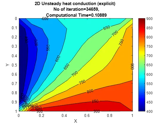
OUTPUT:

2)Implicit method

`T_(i,j)^(n+1)=T_(i,j)^n+K*(T_(i-1,j)^(n+1)+T_(i+1,j)^(n+1)+T_(i,j-1)^(n+1)+T_(i,j+1)^(n+1)-4T_(i,j)^(n+1))`

`(1+4K)*T_(i,j)^(n+1)=T_(i,j)^n+K*(T_(i-1,j)^(n+1)+T_(i+1,j)^(n+1)+T_(i,j-1)^(n+1)+T_(i,j+1)^(n+1))`

`T_(i,j)^(n+1)=(1/(1+4k))*(T_(i,j)^n+K*(T_(i-1,j)^(n+1)+T_(i+1,j)^(n+1)+T_(i,j-1)^(n+1)+T_(i,j+1)^(n+1))`

`T_(i,j)^(n+1)=((T_(i,j)^n)/(1+4k))+(K/(1+4k))*(T_(i-1,j)^(n+1)+T_(i+1,j)^(n+1))+(K/(1+4k))*(T_(i,j-1)^(n+1)+T_(i,j+1)^(n+1))`

Thus we can bifercate the equation in 3 parts to make it simple,

`T_(i,j)^(n+1)=Term1+Term2+Term3`

thus the RHS terms are all unknown therefore it has to be solved using iterative methods

1)Jacobi method

2)Gauss sedal

3)SOR

MATLAB CODE:

close all
clear all
clc
%solving 2D heat conduction equation
%delT/delt=alpha(d^2t/dx^2+d^2t/dy^2)

%inputs
nx=10;
ny=10;
x=linspace(0,1,nx);
y=linspace(0,1,ny);
dx=x(2)-x(1);
dy=y(2)-y(1);
[X,Y]=meshgrid(x,y)
tol=1e-4;
error=9e9;
alpha=1.5;
T=zeros(nx,ny);
omega=1.5;  %For SOR
nt=14000; %no of time step
dt=10; % time step 

%Assigning BC
T(:,1)=400; %left BC
T(:,nx)=800; %right BC
T(1,:)=600; %top BC
T(ny,:)=900; %bottom BC
%corner points
T(1,1)=500;
T(nx,1)=650;
T(1,ny)=700;
T(nx,ny)=850;

%CFL number will be same as nx=ny
K1=alpha*(dt/(dx)^2);
K2=alpha*(dt/(dy)^2);

%creating a copy of T
Told=T;
T_prev_dt=T;

%decide to go for jacobi or GS or SOR (1 or 2 or 3) 
iterative_solver=1;

%jacobi method
tic
    if iterative_solver==1
        jacobi_iter=1;
        for l=1:nt
        while(error > tol)
            for i=2:nx-1
                for j=2:ny-1
                    x1=1/(1+2*K1+2*K2);
                    x2=x1*K1;
                    x3=x1*K2;
                    Term1=(Told(i-1,j)+Told(i+1,j));
                    Term2=(Told(i,j-1)+Told(i,j+1));
                    T(i,j)=((T_prev_dt(i,j)*x1)+(x2*Term1)+(x3*Term2));
                end
            end
        error= max(max(abs(Told-T)));
        Told=T;
        jacobi_iter=jacobi_iter+1;
        end
        T_prev_dt=T;
        end
       
        F=toc;
        figure(1)
contourf(x,y,T);
[a,b]=contourf(x,y,T);
clabel(a,b);
xlabel('X')
ylabel('Y')
set(gca,'ydir','reverse')
colorbar
colormap(jet)
title_text=sprintf('2D Unsteady heat conduction (implicit) \n No of Jacobi iteration=%d,\n Computational Time=%0.5f',jacobi_iter,F);
title(title_text)
    end
    
 %gauss seidal
 tic
    if iterative_solver==2
        gs_iter=1;
        for l=1:nt
        while(error > tol)
            for i=2:nx-1
                for j=2:ny-1
                    x1=1/(1+2*K1+2*K2);
                    x2=x1*K1;
                    x3=x1*K2;
                    Term1=(T(i-1,j)+Told(i+1,j));
                    Term2=(T(i,j-1)+Told(i,j+1));
                    T(i,j)=((T_prev_dt(i,j)*x1)+(x2*Term1)+(x3*Term2));
                end
            end
        error= max(max(abs(Told-T)));
        Told=T;
        gs_iter=gs_iter+1;
        end
        T_prev_dt=T;
        end
        F=toc;
        figure(1)
contourf(x,y,T);
[a,b]=contourf(x,y,T);
clabel(a,b);
xlabel('X')
ylabel('Y')
colorbar
colormap(jet)
set(gca,'YDIR','reverse')
title_text=sprintf('2D Unsteady heat conduction (implicit) \n No of gauss seidal iteration=%d,\n Computational Time=%0.5f',gs_iter,F);
title(title_text)
    end
    
 %SOR 
 tic
    if iterative_solver==3
        sor_iter=1;
        for l=1:nt
        while(error > tol)
            for i=2:nx-1
                for j=2:ny-1
                    x1=1/(1+2*K1+2*K2);
                    x2=x1*K1;
                    x3=x1*K2;
                    Term1=(T(i-1,j)+Told(i+1,j));
                    Term2=(T(i,j-1)+Told(i,j+1));
                    T_gs(i,j)=((T_prev_dt(i,j)*x1)+(x2*Term1)+(x3*Term2));
                    T(i,j)=((1-omega)*Told(i,j))+omega*T_gs(i,j);
                end
            end
        error= max(max(abs(Told-T)));
        Told=T;
        sor_iter=sor_iter+1;
        end
        T_prev_dt=T;
        end
        F=toc;
        figure(1)
contourf(x,y,T);
[a,b]=contourf(x,y,T);
clabel(a,b);
xlabel('X')
ylabel('Y')
colorbar
colormap(jet)
set(gca,'YDIR','reverse')
title_text=sprintf('2D Unsteady heat conduction (explicit) \n No of SOR iteration=%d,\n Computational Time=%0.5f',sor_iter,F);
title(title_text)
    end

OUTPUT:

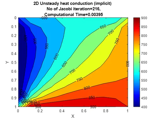
1) Jacobi

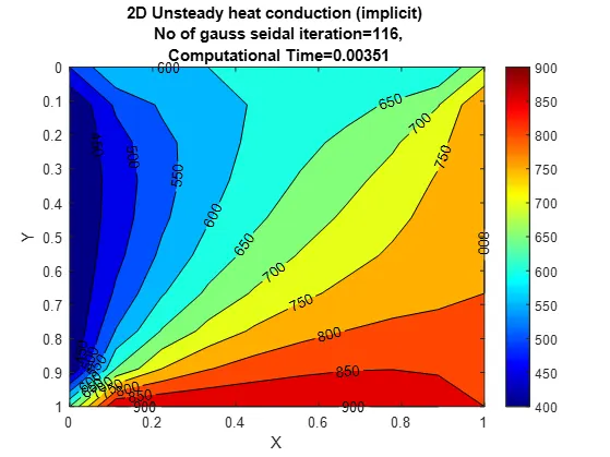
2) Gauss seidel

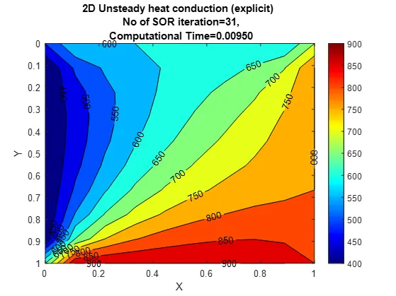
3) SOR

CONCLUSION:

	Method	No of iteration	Simulation time(s)
Steady Implicit	Jacobi	217	0.01446
	Gauss-Seidel	117	0.00267
	SOR	30	0.00349
Unsteady Explicit		34659	0.10889
Unsteady Implicit	Jacobi	216	0.00395
	Gauss-Seidel	116	0.00351
	SOR	31	0.0095

Thus we can conclude that,

• Jacobi has the highest number of iteration in an implicit scheme, while SOR has the lowest.
• The unsteady explicit solved equation converges at 34659 iterations later.
• If the Jacobi method converges in 217 iterations for steady-state heat conduction equation then gauss seidel converges in 117 i.e almost half the iteration of Jacobi this is because gauss seidel uses same equation as Jacobi only the difference is the new values of T are updated wherever it is possible.
• Further, SOR converges in only 30 iterations as it uses over relaxation term `omega` this omega should carefully be selected as if it is below 1, then iterations will be more than the Jacobi method while if it greater than or equal 2 it will blow away the solution. Also, it should be noted that increasing `omega` more than a particular value in the current case 1.5 will oscillate the solution i.e the solution converges in less or more number of iteration from 1.5 to 2.
• Faster solution based on the number of Iteration follows the general trend of SOR > Gauss-seidel > Jacobi.
• The above trend is similar for both Steady and Unsteady implicitly solved equations.