Week 9 - FVM Literature Review

AIM

Write a literature review on Finite Volume Method (FVM)

INTRODUCTION

FVM is a method of solving and presenting the PDE in the form of algebric equations. It conversts volume integrals is converted to the surface integrals in a PDE with a divergence term with the help of divergence theorem. The terms can be represented as the fluxes entering and leaving the volume. This method is conservative as the flux leaving and entering the volume are identical. This method is very compatible with complew geometry and unstrucured meshes. The volume surrounding the each node in a mesh is reffered as the 'Finite Volume'.

Finite volume methods can be compared and contrasted with the finite difeerence methods, which approximate derivatives using nodal values, or finite element methods, which create local approximations of a solution using local data, and construct a global approximation by stitching them together. In contrast a finite volume method evaluates exact expressions for the average value of the solution over some volume, and uses this data to construct approximations of the solution within cells.

In CFD we can notice that the following solver methods can be defined:-

1) Finite Difference Method
2) Finite Element Method
3) Finite Volume Method

Method of using Finite Volume Method to solve a problem:

1) We first write equations for a defined volume and not for a single node.

2) Then we apply the Mathematical Techniques to solve the equations defined for the grid.

3) We can say that the FVM method works on the princilple of conversation.

Steps for Discretizing the finite volume:-

1) Write the governing equation in the integral form.
2) Apply gauss divergence theorem.
3) Take suitable methods to calculate the flux terms.

Solving 1D linear heat conduction equation using Finite Volume Method

Defining the 1D grid-

The general Governing equation or the conservative equation given by;

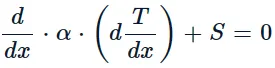
Here, S- source term which is responsible for the heat generation.

alpha - function of temperature.

Now, Let's consider a small volume from this given control volume, for which the governing equation is given by;

Then simplifing the above equation and considering (w,e) in the control volume;

To find the dT/dx value at the above hilighted points, we can use Taylor series for approximation.

On solving the above equation we get,

Here,

- source term ; A- face area; dV= volume.

For source term in CFD, the source term that is going to added in a cell if it is actually the function of the temperature then linearisation is done to the source term.

On linearising this source term we get;

Su+Sp⋅Tp

The above equation consist of a constant term and states that source term is the function of temperature.

The main equation says that [Heat flux out ] - [Heat flux inn] + Source term = 0.

Hence FVM is said to conserve quantity better as in the derivation we are considering the equations for controlled volume and finally getting results in the form that is conservative.

The Interpolation Schemes for FVM:

1) Upwind Interpolation Scheme
2) Linear Interpolation Scheme
3) Quadratic upwind Interpolation Scheme
4) Hybrid,TVD and ENO Interpolation Scheme

The Upwind Interpolation Scheme -

This method is used mainly for the convection dominant problems. Velocity for a given point ,the direction of that particular velocity that determines the variables values used in interpolation process. In upwind scheme it make use of nodes that are in the upstream of the given node.

It is used to calculate the approximate value of the variable(f) at the east face of the control volume, the equation is given by;

This scheme is almost similar to the forward difference approximation or a backward difference approximation based on the flow direction.

We know that, when calculating gradience, we need to have those values bounded, so that they dont jump. Hence this approximation satisfies the boundness condition.

Linear Interpolation Scheme -

Linear interpolation is the method of generating new data points with a range of a discrete set of known data points.

Where,

The linear Interpolation scheme is same as the central difference formula that we considered for the first order derivative. So this scheme is also known as the central difference scheme.

Generally it is used to solve the integrated convection-diffusion equation.

It leads to a easy approximation for the evaluation of gradients that are required for evaluation of diffusive fluxes.

CDS is a second order accurate and may produce oscillatory solutions i.e here if the grid spacing is very large we can find oscillatory solutions. It is bascially a first order, as we refine the grid then accuracy is close to the second order.

Quadratic upwind Interpolation Scheme -

In CFD it is called as QUICK i.e. Quadratic Upstream Interpolation for Convective Kinematics.

QUICK considers the second order derivative term into consideration and ignores the third order derivative term.Hence it is considered as third order accurate.

Now approximate the value of the particular variable at the face centre of the control volume by the quadratic intropolation by using the values at three nearest computational nodes i.e 1 downstream node(D) and two upstream nodes(U, UU) respectively. The equation is given by;

where,

This scheme generally used to solve the convective-diffusion equations using the second order central difference for the diffusion term and for the convection term the scheme is third order accurate in space and first order accurate in time.

Limiation to FVM

• For a convective fluid flow it has been observed that for the low arder schemes are stable but unstable during discontunity or shocks, where as higher order schemes unbalanced or unstable in nature because they show high oscillations and sharp changes in the solution .
• These are used in high resolution schemes.These help in limitting the solution gradient near shocks and discontinuities. Objective of implementing flux limiter schemes is to control the spatial derivativesto the realistic values.
• The limiter function is greater than or equal to zero ,i.e. when the limitter is equal to zero then the flux is represented by low resolution schemes.Similarly if the limitter is equal to 1 (smooth solution), it is represented by high resolution schemes.
• Flux limiters are also called as slope limiters as they have same mathematical form and they can help in limiting the solution gradient near shocks and discontinuities.
• The flux limitter is used when the limiter acts on the system fluxes and slope limiter is used when the limitter acts on the system(like pressure and velocity).
• This factor are selected as per the given problem and the scheme used for the solution.