Week 9 - FVM Literature Review

Objective

What is Finite Volume Method(FVM), write down the major differences between FDM & FVM. Also, describe the need for interpolation schemes and flux limiters in FVM. You can use the 1D linear heat conduction equation as an example.

Solution

There are four widely used numerical method-based solutions for the Navier Stokes Equations in computational fluid dynamics (CFD). There are 4 of these:

1. Finite Element Method (FEM)
2. Boundary Element Method (BEM)
3. Finite Volume Method (FVM)
4. Finite Difference Method (FDM)

The finite-difference and finite-volume approach of efficient CFD technology has grown in popularity and has been used for significantly longer periods of time.

Finite Difference Method (FDM)

In order to truncate the computational domain, boundary constraints are required. They stand in for the aspect of contact with the outside world that we do not want our simulation to contain. We can easily encounter issues while using borders to define the boundary conditions when using the finite-difference approach. Based on the differential form of the PDE that has to be solved, the finite-difference technique is the most straightforward way for discretizing. We take into account a location in space where the finite-difference equations are used to substitute the continuum form of the equations.

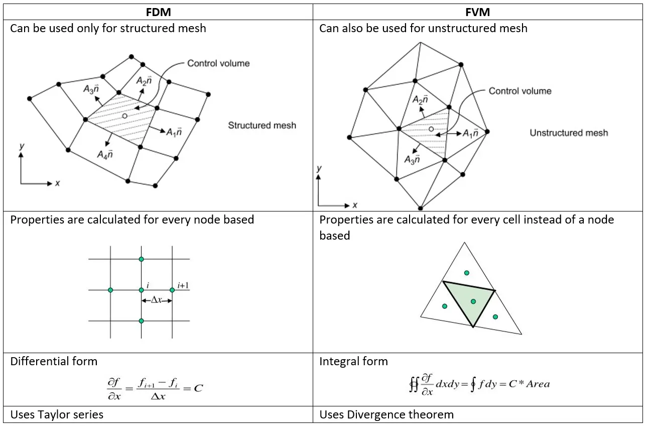
The computational domain is often split into hexahedral cells (the grid), and the solution is determined at each nodal point. This is how the finite-difference approach is commonly described. and extremely effective problem-solving techniques may be based on this fact. For extremely large-scale simulations on supercomputers, regular grids are helpful. Therefore, the approach is more often used to models that are rectangular or block-shaped rather than irregular CAD geometries.

Simulations of the space shuttle and Formula 1 cars' computational fluid dynamics (CFD) are two examples. The finite-difference approach makes treating material discontinuities more challenging. Additionally, it does not lend itself to "adaptive mesh refinement" or local grid refinement. This may be required to address local, quick fluctuations in solutions, such as those that occur near a complicated shape's corner, as was previously explained.

However, efficient implementations are significantly simpler than for finite-volume techniques if we can fit the simulation in a rectangle or box-shaped geometry using a regular grid. If the boundary-condition issue with curved borders can be solved, the approach produces extremely effective and superior results. Due to the fact that the finite-difference approach is specified dimension by dimension, raising the "element order" to get higher-order accuracy is simple.

Finite Volume Method (FVM)

Similar to the finite-differencing approach, the finite-volume method first divides the CAD model into extremely tiny yet finite-sized pieces of geometrically straightforward forms. Apart from this, there are many other significant differences between the finite-volume approach and the finite-differencing method, starting with the terminology used for the elements, which is changed to cells.

A discretization using the finite volume method (FVM) can manage discontinuities in solutions since it is based on the integral form of the PDE that has to be solved (such as conservation of mass, momentum, or energy). The PDE is expressed in a way that allows it to be solved for a certain finite volume (or cell). The governing equations are then solved for each volume after discretizing the computing domain into finite volumes. Calculating fluxes is crucial in FVM because the resultant system of equations often incorporates fluxes of the conserved variable.

The advantage of the finite-volume technique is that just the cell borders need to be evaluated for flow. This also applies to nonlinear issues, making it much more potent for resolving (nonlinear) conservation rules that pop up in transportation-related issues.

The mesh surrounding an important corner may be improved to boost the local accuracy of the finite-volume approach there. However, it is difficult to create higher order functions that approach the answer when utilising the finite-volume technique. In comparison to the finite-difference approach, the finite-volume method has this drawback.

This approach has a fundamental benefit over FDM in that it does not call for the usage of structured grids, and the internal effort to transform the provided mesh into a structured numerical grid is entirely avoided. The approximate solution that is produced is discrete, much as in FDM, however the variables are often located at cell centres rather than nodal points. There are additional face-centered finite volume algorithms, thus this isn't necessarily the case. In any scenario, interpolation is used to acquire the values of field variables at non-storage places, such as vertices.

Interpolation schemes:

The values of the variable must be at locations other than the computational nodes of the control volume in order to approximate surface and volume integrals. Utilizing interpolation formulas, values are derived at these places.

Interpolation methods:

Upwind interpolation

Linear interpolation

Quadratic upwind interpolation

Hybrid, TVD and ENO interpolation schemes

Upwind interpolation

We utilise the node upwind or upstream of the specified node, as the name implies. It is used in cases when convection-dominated issues exist.

For estimating the value of a variable f at the east face of a control volume, the upwind interpolation is provided by

`f_e={(f_p, if(upsilon.eta)_e>0) ,(f_e,if(upsilon.eta)_e<0):}`

Depending on the direction of the flow, this interpolation approach is comparable to utilising either the forward difference method or the backward difference method. The only approximation that never yields oscillatory solutions and unconditionally meets the boundedness criteria regardless of velocity or grid spacing is the UDS.
UDS has the drawback of being numerically diffusive.
If flow is perpendicular to the grid, numerical diffusion in multidimensional problems is amplified.

The variables' peaks or abrupt changes will be obscured.

First-order accuracy only. Therefore, extremely tiny grids are necessary to get precise results.

Linear interpolation

The two closest computational nodes at point e are used to approximate the value of the variable at the control volume face centre. This is the same as a central difference first-order derivative method. It is accurate to second order and generates oscillatory solutions.

by linearly interpolating the values at the two closest computational nodes, approximate values of the variable at the control volume face centre.

`f_e=f_Elambda_e+f_P(1-lambda_e)`

where

`lambda_e=(x_e-x_p)/(x_E-x_P)`

Flux limiter:

The higher-order schemes are unstable in nature and exhibit oscillations close to the sites of discontinuity or shocks, while low-order schemes for convective fluid flow are typically stable but extremely dissipative in nature at these points. High-Resolution Schemes are thought to be very accurate and oscillation-free. The higher-order schemes are unstable in nature and exhibit oscillations close to the sites of discontinuity or shocks, while low-order schemes for convective fluid flow are typically stable but extremely dissipative in nature at these points. High-Resolution Schemes are thought to be very accurate and oscillation-free.

In order to make the scheme TVD, we must constrain or limit the range of possible values of the additional convective flux `f_e=f_p+(1/2)psi(r)(f_E-f_P)`

It was first included to raise the order of the plan. As a result, the function `psi(r)` is referred to as a flux limiter function.

The higher-order and lower-order schemes are fine-tuned using flux limiter functions such that the resultant scheme provides higher-order accuracy in the smooth area of the flow and retains first-order accuracy close to shocks and discontinuities. A TVD scheme is used for such a plan.

`F(u_(i+(1/2)))=f^(low)(i+1/2)-psi(r_i)(f^(low)(i+1/2)-f^(high)(i+1/2))`

`F(u_(i-(1/2)))=f^(low)(i-1/2)-psi(r_i-1)(f^(low)(i-1/2)-f^(high)(i-1/2))`

where

`f^(low)=`low precision flux (first order)

`f^(high)=`high precision flux (higher-order)

Conclusion

The Finite Volume Method (FVM) is a particularly effective method for resolving CFD issues. We can resolve a variety of CFD issues with the aid of suitable interpolation algorithms and the precise use of flux limiters in the event of any current discontinuities. Although it could be challenging to develop and apply it in the computer, it has the extra benefit of being sturdy.