Week 9 - FVM Literature Review
Aim: What is Finite Volume Method(FVM), write down the major differences between FDM & FVM. Also, describe the need for interpolation schemes and flux limiters in FVM. You can use the 1D linear heat conduction equation as an example.
1. What is Finite Volume Method (FVM)?
Ans- Finite volume method (FVM) is based on an unstructured (e.g. triangular) mesh. Therefore, it is suitable for irregular and complex geometries. FVM has another advantage over FEM for fluid mechanic problems. So far, the numerical methods that we presented have been based on PDEs. By contrast, FVM is based on the integral form of the conservation laws, rather than their differential form. This leads to more accuracy/stability, especially for sharp gradients (i.e. large derivatives) inside a domain, which is also called shock-capturing property. To explain this more clearly, as we mentioned before, the dynamics of flow can be described by conservation of mass, momentum, and energy. These conservation laws can be written as a system of PDEs. Alternatively, conservation laws can be expressed by integral equations (i.e. Reynolds transport theorem).
For instance, the differential form of the continuity equation can be written as
where u, v, and w are the components of flow velocities in the x, y, and z directions, and ρ is the density. The integral form of continuity for a control volume (or a finite volume) can be written as
where V is the control volume, S is the control surface, u = (u, v, w), and S is the surface vector.
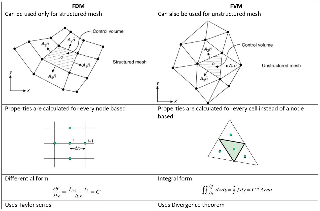
Therefore, the change of mass inside a control/finite volume plus the net mass fluxes through the control surface should be zero. In FVM, the domain is first discretized into a number of nonoverlapping finite volumes or cells (see Fig. 8.12 as an example). Usually, these finite volumes are triangles (2D) or prisms (3D). Next, conservation laws are applied to each individual cell to form enough algebric equations, which can be solved to compute the state variables.
2. Write down the major differences between FDM & FVM.
Ans-
- Finite Difference method (FDM): This is one of the numerical techniques which is used to find the approximate solution of the Differential equations. First, these differential equations are converted into a system of algebraic equations by using Taylor expansion and it is useful for the rectangular domain only. This method fails to formulate the mathematical model for complex geometry.
- Finite Element Method (FEM): Finite element method helps us to solve the Differential equation within the complex domain. First, this method is used to form the differential equation into its weak formulation, and then under some technical spaces its solves the model into its approximate value. This method is better than the FDM.
3. Describe the need for interpolation schemes and flux limiters in FVM.
Ans- The approximations of surface and volume integrals require values of the variable at location other than the computational nodes of the control volume. Values at these locations are obtained using interpolation formulae.
- Upwind interpolation
- Linear interpolation
- Quadratic upwind interpolation
- Hybrid, TVD and ENO interpolation schemes
1. Upwind interpolation (UDS)
As the name indicates that we use the node in the upwind or upstreame of the given node.It is used in case of convection dominated problems.The upwind interpolation for approximating the value of a variable f at the east face of a control volume is given by
fe={fp,if(v.n)e>0fE,if(v.n)e<0fe={fp,if(v.n)e>0fE,if(v.n)e<0
This interpolation scheme is equivalent to using Forward difference method or backward difference method depending on the flow direction.
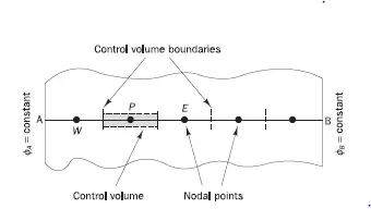
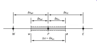
If the flow is along −X-X direction, then the values for this at the interface is given by
for v>0;ui−12≈ui−1;ui+12≈uiv>0;ui-12≈ui-1;ui+12≈ui
Ic≈vui−ui−1ΔxIc≈vui-ui-1Δx which is equivalent to Backward Difference aScheme
If the flow is along +X+X direction, then the values for this at the interface is given by
for v>0;ui−12≈ui−1;ui+12≈uiv>0;ui-12≈ui-1;ui+12≈ui
Ic≈vui+1−uiΔxIc≈vui+1-uiΔx which is equivalent to Forward Difference Scheme
It is said to be equivalent because all these three methods are of order of accuracy 1.
2. Linear interpolation (CDS)
Approximate values of the variable at the control volume face centre by the linear interpolation of the values at the two nearest computational nodes.It is simple and most widely used`The linear interpolation is equivalent to the use of central difference formula of the firs order derivative and hence this scheme is aslo termed as Central Differencing Scheme(CDS).
fe=fEλe+fp(1−λe)fe=fEλe+fp(1-λe)
where λe=xe−xpxE−xPλe=xe-xpxE-xP
Average interface values are given by
ui−12≈ui−1+ui2ui-12≈ui-1+ui2 and ui+12≈ui+ui+12ui+12≈ui+ui+12
Ic≈v.ui+1−ui−12ΔxIc≈v.ui+1-ui-12Δx which is equivalent to CDS
It is said to be equivalent because both these methods are of order of accuracy 2`
3. Hybrid interpolation scheme
It is the blend of UDS and CDS. The hybrid difference scheme exploits the favourable properties of the
upwind and central differencing schemes. It switches to upwind differencing when central differencing produces inaccurate results at high Pe numbers.
The scheme is fully conservative and since the coefficients are always positive it is unconditionally bounded. It satisfies the transportiveness requirement by using an upwind formulation for large values of Peclet number.
fe=γfCDS+(1−γ)fUDSfe=γfCDS+(1-γ)fUDS
4. Quadratic Upwind Interpolation for convective kinematics (QUICK)
It approximates the values of the variable at the CV face centre by Quadratic Interpolation of the values at three nearest computational nodes (1 Down stream node D & 2 Up stream nodes U , UU).
Quadratic - As it uses 3 nodes
Upwind - As it uses two upstreams
Convective Kinematics - As it is used for convective domain problems
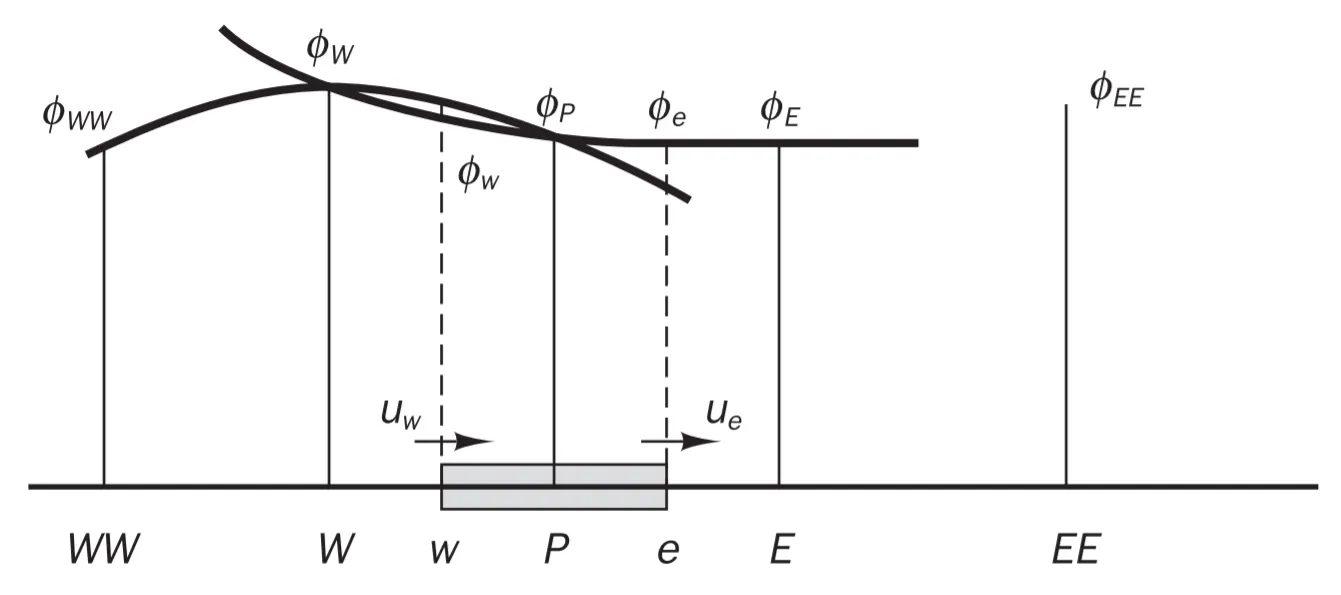
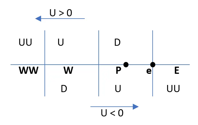
fe=fE+g1(fD−fU)+g2(fUU−fU)fe=fE+g1(fD-fU)+g2(fUU-fU)
Where,
g1=(xe−xU)(xe−xUU)(xUU−xU)(xUU−xD)g1=(xe-xU)(xe-xUU)(xUU-xU)(xUU-xD)
g2=(xe−xU)(xe−xD)(xUU−xU)(xUU−xD)g2=(xe-xU)(xe-xD)(xUU-xU)(xUU-xD)
5. Total variation diminishing scheme (TVD)
The fact that the QUICK scheme and other higher-order schemes can give undershoots and overshoots has led to the development of second-order schemes that avoid these problems. The class of TVD (total variation diminishing) schemes has been specially formulated to achieve oscillation-free solutions and has proved to be useful in CFD calculations.
TVD schemes are designed to address this undesirable oscillatory behaviour of higher-order schemes. In TVD schemes the tendency towards oscillation is counteracted by adding an artificial diffusion fragment or by adding a weighting towards upstream contribution.
It is 2nd order accurate.
fe=fp+12ψ(r)(fE−fP)fe=fp+12ψ(r)(fE−fP)
where,
ψ(r) is called a flux limiter function
where,
r=ui−ui−1ui+1−uir=ui-ui-1ui+1-ui
Flux limiter:
For convective fluid flow, it is ovservedthat low order schemes are usually stable but quite dissipative in nature around the points of discontinuity or shocks while the higher order schemes are unstable in nature and show oscillations in the vicinity of dinscontinuity or shocks. Highly accurate and oscillation free schemes are known as High Resolution Schemes.
In order to make the scheme TVD, we must constrain or limit the range of possible values of the additional convective flux i.e
fe=fp+12ψ(r)(fE−fP)fe=fp+12ψ(r)(fE−fP),
which was originally introduced to make the scheme higher-order. Hence, the function ψ(r)ψ(r) is called a flux limiter function.
Flux Limiter functions are used to fine tune the higher order and lower order schemes in such a way that the resulting scheme gives a higher order accuracy in the smooth region of the flow and maintains first order accuracy in the vicinity of shocks and discontinuities. For such a scheme TVD scheme is employed.
F(ui+12)=flow(i+12)−ψ(ri)(flow(i+12)−fhigh(i+12))F(ui+12)=flow(i+12)-ψ(ri)(flow(i+12)-fhigh(i+12))
F(ui−12)=flow(i−12)−ψ(ri−1)(flow(i−12)−fhigh(i−12))F(ui-12)=flow(i-12)-ψ(ri-1)(flow(i-12)-fhigh(i-12))
Conclusion: