Week 3 - Solving second order ODEs
AIM - program in Matlab that will simulate the pendulum motion in 2nd order ODE.
OBJECTIVE:
- Write a program in Matlab that will simulate the pendulum motion.
- write a program that solves the following ODE. This ODE represents the equation of motion of a simple pendulum with damping.
THEORY:
- A pendulum is a weight suspended from a pivot so that it can swing freely. When a pendulum is displaced sideways from its resting, equilibrium position, it is subject to a restoring force due to gravity that will accelerate it back toward the equilibrium position.
-
A simple pendulum consists of a mass m hanging at the end of a string of length L. The
period of a pendulum or any oscillatory motion is the time required for one complete
cycle, that is, the time to go back and forth once.
EQUATION:
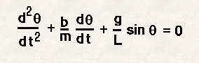
where,
g = gravity in m/s2,
L = length of the pendulum in m,
m = mass of the ball in kg,
b=damping coefficient.
DATA TO BE USE:
L=1 metre,
m=1 kg,
b=0.05.
g=9.81 m/s2
CODES
- FUNCTION CODE
function [dtheta_dt] = ode_func(t,theta,b,g,l,m)
theta1 = theta(1);
theta2 = theta(2);
dtheta1_dt = theta2;
dtheta2_dt = -(b/m)*theta2 - (g-1)*sin(theta1);
dtheta_dt = [dtheta1_dt;dtheta2_dt]
end
EXPLANATION - A function is creatd first namely "ode_func" to use it further in the main program.
Inside the function, we solved the equation and got the resultant as "dtheta_dt".
- MAIN CODE
clear all
close all
clc

%INPUTS
b = 0.05;
g = 9.81;
l = 1;
m = 1;

%initial condition
theta_0 = [0;3];

%time points
t_span = linspace(0,50,100);

%solve ODE by clling ODE function
[t,results] = ode45(@(t,theta) ode_func(t,theta,b,g,l,m),t_span,theta_0);

%plotting
figure(1);
subplot(1,2,1);
plot(t,results(:,1),'linewidth',1,'color','r');
title("Angular displacement vs time")
xlabel('angular displacement')
ylabel('time')
hold on
subplot(1,2,2);
plot(t,results(:,2),'linewidth',1,'color','b');
title("Angular velocity vs time")
xlabel('angular velocity')
ylabel('time')
grid on;

%animation of pendulum
%counter variable= C
C=1
for a=1:length(results(:,1))
    x0 = 0;
    y0 = 0;
    x1=l*sin(results(a,1))
    y1=-l*cos(results(a,1))

figure(2)
title('motion of simple pendulum');
plot([-1 1],[0 0],'linewidth',5,'Color','b')
hold on
line([0 x1],[0 y1],'linewidth',3,'Color','r')
hold on
plot(x1,y1,'Marker','o','MarkerSize',20,'MarkerEdgeColor','r','MarkerFaceColor','g')
hold on
axis([-2,2,-3,1])

grid on;

pause(.006);
hold off;

    %storing frames in m
    M(C)=getframe(gcf);
    C=C+1;
  end

%creatig videofile for m
movie(M)
videofile=VideoWriter('pendulum.avi','Uncompressed AVI')
open(videofile)
writeVideo(videofile,M)
close(videofile)
EXPLANATION-
Step- 1
%INPUTS
b = 0.05;
g = 9.81;
l = 1;
m = 1;
expanation- All the inputs are given according to the question.
Step -2
%initial condition
theta_0 = [0;3];
%time points
t_span = linspace(0,50,100);
%solve ODE by clling ODE function
[t,results] = ode45(@(t,theta) ode_func(t,theta,b,g,l,m),t_span,theta_0);
explanation- Initial condition is given and through "ode45", the function "ode_func" is called.
step-3
%plotting
figure(1);
subplot(1,2,1);
plot(t,results(:,1),'linewidth',1,'color','r');
title("Angular displacement vs time")
xlabel('angular displacement')
ylabel('time')
hold on
subplot(1,2,2);
plot(t,results(:,2),'linewidth',1,'color','b');
title("Angular velocity vs time")
xlabel('angular velocity')
ylabel('time')
grid on;
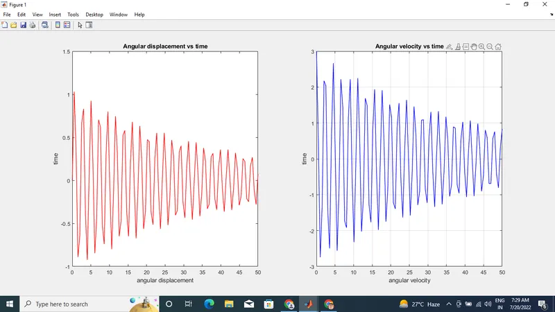
explanation - plotting of 2 graphs are done, i.e (i)- "Angular displacement vs time" & (ii)- ("Angular velocity vs time").
For plotting both the graph at the same figure we have used "subplot".
step-4
%animation of pendulum
%counter variable= C
C=1
for a=1:length(results(:,1)) ##("for" loop started)
x0 = 0;
y0 = 0;
x1=l*sin(results(a,1))
y1=-l*cos(results(a,1))
explanation- for animation, the counter value, initial value and the end value is given.
figure(2)
title('motion of simple pendulum');
plot([-1 1],[0 0],'linewidth',5,'Color','b')
hold on
line([0 x1],[0 y1],'linewidth',3,'Color','r')
hold on
plot(x1,y1,'Marker','o','MarkerSize',20,'MarkerEdgeColor','r','MarkerFaceColor','g')
hold on
axis([-2,2,-3,1])
grid on;
pause(.006);
hold off;
explanation- plotting of figure 2 (which is an animation) is done. Here, the plotting of horizontal wall,the string and the ball is done.
%storing frames in m
M(C)=getframe(gcf);
C=C+1;
explanation- The frames are stored.
end ##("for" loop end)
step-5
%creatig videofile for m
movie(M)
videofile=VideoWriter('pendulum.avi','Uncompressed AVI')
open(videofile)
writeVideo(videofile,M)
close(videofile)
Explanation- The video file for animation is created.
- SYNTAX OF ode45
[t,y] = ode45(@odefun,tspan,y0,options)
[t,y,te,ye,ie] = ode45(@odefun,tspan,y0,options)
sol = ode45(__)
OUTPUT:
- GRAPH
- ANIMATION LINK
ERRORS-
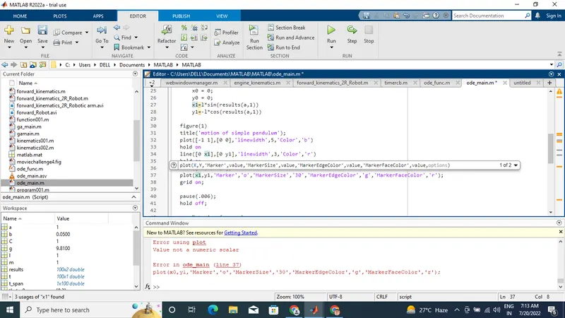
- Forgot to use "hold on" after plotting the ball. That's why the error was coming.