Week 9 - FVM Literature Review
(FVM) Finite Volume Method:-
The Finite Volume Method (FVM) is a way to write partial differential equations as algebraic equations and solve them.
In this method, the volume is integrated into a partial differential equation with a divergence term, and the divergence theorem is used to turn the volume integrals into surface integrals. Then, the fluxes at the surfaces of each finite volume are calculated based on these terms. These methods are conservative because the flux going into a given volume is the same as the flux going out of the volume next to it.
"Finite volume" refers to the small area around each node point on a mesh.
The finite volume method is useful because it is easy to write down and can be used with unstructured meshes. This method is used in many computational fluid dynamics packages.
What's different about FDM and FVM:-
The discretization of a PDE using the finite difference method (FDM) depends on how it is written in differential form. Each derivative is replaced with a formula for an approximation of the difference, which can usually be gotten from a Taylor series expansion. Usually, the computational domain is broken up into a grid of six-sided cells, and the solution will be found at each nodal point.
A finite volume method (FVM) is a way to break up a PDE that needs to be solved (eg. conservation of mass, momentum, or energy). The PDE is written in a way that makes it possible to solve it for a given finite number of cells. The computational domain is broken up into small volumes, and then the governing equations are solved for each volume. Most of the time, the system of equations that results includes fluxes of the variables that stay the same. Because of this, flux calculations are very important in FVM.
The main benefit of this method over FDM is that it doesn't need structured grids, and there's no need to change the mesh into a structured numerical grid internally.
Schemes of interpretation:- Surface and volume integrals may need values of the variable in places other than the computational nodes of the CV in order to be approximated. Interpolation formulas are used to find the values at these points.
Upwind Interpolation:-
Upwind interpolation (UDS) is a way to estimate the value of a variable on the east side of a control volume.

This method of interpolation is the same as using a finite difference approximation in either direction (depending on the flow direction).
LINEAR INTERPOLATION (CDS):-
We can get a good idea of the value of the variable at the centre of the CV face by taking the values at the two closest computational nodes and interpolating them. So, the approximate value of the variable at point e on a Cartesian grid is:
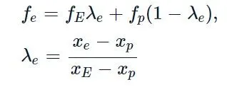
This scheme is also called the central difference scheme because linear interpolation is the same as using the central difference formula of the first-order derivative (CDS). This plan is accurate to the second order and may lead to solutions that move back and forth.
QUADRATIC UPWIND INTERPOLATION:- Polynomial fitting can be used to come up with a quadratic upwind interpolation (QUICK) scheme. On a uniform Cartesian grid, the formula for QUICK interpolation is:
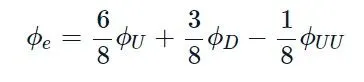
where D is the downstream node, U is the first upstream node, and UU is the second upstream node (E, P, and W or P, E, and EE depending on the flow direction). The QUICK method is accurate to the third order, but it tends to go in and out of sync.
Flux limiters:-
Flux limiters are used in the high-resolution scheme that scientists and engineers use to solve problems, especially in fluid dynamics, which is described by PDEs. They are used in a high-resolution scheme like the MUSCL scheme to avoid the spurious oscillation that would happen with a high order spatial discretization scheme if the solution domain had shocks, breaks, or sharp changes. When flux limiters and a good high-resolution scheme are used together, the total variation of the solution goes down (TVD).
The main goal of making flux limiters is to limit the spatial derivatives to values that make sense for scientific and engineering problems. Usually, this means values that can be physically realised and have meaning. They are used in the high-resolution scheme to solve problems described by PDEs. However, they only work when there are sharp wavefronts. For waves that change in a smooth way, the flux limiters don't work, and the spatial derivatives can be represented by a high-order approximation without causing oscillations that aren't there.
Think about the below 1D semi-discrete scheme;
where;

represents low-resolution and high-resolution schemes. The flux limiters can then be switched between these schemes based on the gradient near a particular cell.
where,
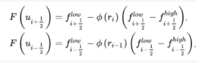
So, when the limiter is equal to zero, the flux is shown by a scheme with a low level of detail. In the same way, a high-resolution scheme is used when the limiter is equal to 1.
Different limiters have different ways of turning on and off, and they are chosen based on the problem and how to solve it.
References:-
https://en.wikipedia.org/wiki/Flux_limiter
Introduction to Computational Fluid Dynamics: The Finite Volume Method"