Project 1 - Parsing NASA thermodynamic data
Aim:
Utilize the data's coefficients to evaluate thermodynamic parameters like Cp, H, and S.
Objective:
Create a function that takes the 14 coefficients as input and computes the enthalpy, entropy, and specific heats for each species in the data file. Determine each species' molecular weight and show it in the command window. Plot the Cp, Enthalpy, and Entropy values for each species' unique local temperature range (low to high temperature). Plots should be saved as pictures with descriptive file names and placed in distinct folders for each species. All of these need to be produced automatically. The primary programme you'll provide will create Cp, H, and S graphs using the "THERMO.dat" file as input.
Theory:
Specific Heat: The amount of energy needed to raise a substance's temperature by one degree for every unit of mass is known as its specific heat or Cp.
Enthalpy (H): This unit of measurement for energy in thermodynamic systems equals the sum of the system's internal energy and the volume and pressure products.
Entropy: Entropy is a measurement of molecular disorder or unpredictability.
CODE explanation:
First, we'll type in the parameter R, then open the THERMO.dat file and use the fopen command to read from it.
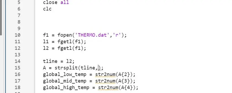
Then, we'll read the first THERMO using the fgetl command. After that, we'll read the temperature file, split the temperatures using the strsplit command to turn them into a cell array, and then use the str2num command to find the low, high, and average temperatures.
Then, we'll use the linspace command to set a temperature range. Then, we use the fgetl command inside a loop to skip over command lines in the data file.
Now, we'll run the loop to find 53 elements in the data file by assigning the fgetl command and then splitting them into the cell array to find the species line, then the species name, and then the number of temperatures in the species line.
The next line was then read. To read the coefficient from the data file, we will first find the 'E' string using the strfind command to find the numbers before and after the coefficients. We will then find the other 14 coefficients and turn them from strings to numbers.
The first 7 coefficients are for higher temperatures, and the second 7 coefficients are for lower temperatures. Now, we will define the Specific heat Cp, Entropy S, and Enthalpy H functions to find these parameters using these 14 coefficients for lower and higher, and then we will define the Molecular weight W function to find the Molecular weight of the different species. Now, we'll write the Molecular weight.txt file and use fprintf to show all of the species' molecular weights. and then use the fclose command to close the text file.
Now, we use the cd command to change the directory. Then, we use the mkdir command to create a directory folder where we will save our files.
Finally, we use the cd command to change the directory to this folder. Now, we will plot the specific heat, entropy, and enthalpy for each species against its temperature.
We will make different titles for species by using the scanf command in the title command. Then, we'll use the saveas command to save the plots of different species in the directory folder.
Now, we'll change where our main code file runs when we use MATLAB.
Main Program:
% FILE PARSING


clear all
close all
clc


f1 = fopen('THERMO.dat','r');
l1 = fgetl(f1);
l2 = fgetl(f1);

tline = l2;
A = strsplit(tline,' ');
global_low_temp = str2num(A{2});
global_mid_temp = str2num(A{3});
global_high_temp = str2num(A{4});

 for i = 1:3
     P = fgetl(f1);
 end


for j = 1:53

    tline_2 = fgetl(f1);
    B = strsplit(tline_2,' ');

    species = (B{1});
    dot_position = strfind(tline_2, '.');

    local_low_temp = tline_2(dot_position(1)-3 : dot_position(1)+3);
    local_low_temp = str2num(local_low_temp);

    local_high_temp = tline_2(dot_position(2)-4 : dot_position(2)+3);
    local_high_temp = str2num(local_high_temp);

    local_mid_temp = tline_2(dot_position(3)-4 : dot_position(3)+3);
    local_mid_temp = str2num(local_mid_temp);

    species_data_1 = fgetl(f1);
    species_data_2 = fgetl(f1);
    species_data_3 = fgetl(f1);

    D = strfind(species_data_1, 'E');
    E = strfind(species_data_2, 'E');
    F = strfind(species_data_3, 'E');


    % calculating the coefficients

    a1 = species_data_1(1:D(1)+3);
    a2 = species_data_1(D(1)+4 : D(2)+3);
    a3 = species_data_1(D(2)+4 : D(3)+3);
    a4 = species_data_1(D(3)+4 : D(4)+3);
    a5 = species_data_1(D(4)+4 : D(5)+3);
    a1 = str2num(a1);
    a2 = str2num(a2);
    a3 = str2num(a3);
    a4 = str2num(a4);
    a5 = str2num(a5);

    a6 = species_data_2(1:E(1)+3);
    a7 = species_data_2(E(1)+4 : E(2)+3);
    a8 = species_data_2(E(2)+4 : E(3)+3);
    a9 = species_data_2(E(3)+4 : E(4)+3);
    a10 = species_data_2(E(4)+4 : E(5)+3);
    a6 = str2num(a6);
    a7 = str2num(a7);
    a8 = str2num(a8);
    a9 = str2num(a9);
    a10 = str2num(a10);

    a11 = species_data_3(1:F(1)+3);
    a12 = species_data_3(F(1)+4 : F(2)+3);
    a13 = species_data_3(F(2)+4 : F(3)+3);
    a14 = species_data_3(F(3)+4 : F(4)+3);
    a11 = str2num(a11);
    a12 = str2num(a12);
    a13 = str2num(a13);
    a14 = str2num(a14);

    R = 8.314;
    T = linspace(local_low_temp,local_high_temp,500);

    % Calculating the Specific heat, Enthalpy and Entropy calculation


    for i = 1:length(T)               % defining a 'for' loop for the calculation of cp, H & S.

        if T(i) > local_mid_temp
            cp(i) = (a1 + a2.*T(i) + a3.*T(i).^2 + a4.*T(i).^3 + a5.*T(i).^4) .* R;                                      % this equation calculates 'cp' of species for temp>1000
            H(i) = ((a1 + (a2.*T(i))./2 + (a3.*T(i).^2)./3 + (a4.*T(i).^3)./4 + (a5.*T(i).^4)./5) + a6./T(i)).*R.*T(i);  % this equation calculates 'H' of species for temp>1000
            S(i) = (a1.* log(T(i)) + a2 .* T(i) + (a3.*T(i).^2)./2 + (a4.*T(i).^3)./3 + (a5.*T(i).^4)./4 + a7) .* R;     % this equation calculates 'S' of species for temp>1000
        else
            cp(i) = (a8 + a9.*T(i) + a10.*T(i).^2 + a11.*T(i).^3 + a12.*T(i).^4) .* R;                                       % this equation calculates 'cp' of species for temp<1000
            H(i) = ((a8 + (a9.*T(i))./2 + (a10.*T(i).^2)./3 + (a11.*T(i).^3)./4 + (a12.*T(i).^4)./5) + a13./T(i)).*R.*T(i);  % this equation calculates 'cp' of species for temp<1000
            S(i) = (a8.* log(T(i)) + a9 .* T(i) + (a10.*T(i).^2)./2 + (a11.*T(i).^3)./3 + (a12.*T(i).^4)./4 + a14) .* R;     % this equation calculates 'cp' of species for temp<1000
        end
    end


    cd('C:\Users\AK THILAK\AppData\Local\MathWorks\MATLAB\R2022a\O\') % changing the directory.
    mkdir(species);
    cd(species);


     % Plotting the curve between T & cp

    figure(1);
    plot(T,cp, 'linewidth',3, 'Color','b');
    xlabel('Temperature, T [K]');
    ylabel('Specific Heat, cp [kJ/kg.K]');
    grid on;
    title(sprintf('Variation of Specific heat with Temperature for %s', species));
    saveas(figure(1),'cp_vs_T.png');

    % Plotting the curve between T & H.
    figure(2);
    plot(T,H, 'linewidth',3, 'Color','g');
    xlabel('Temperature, T [K]');
    ylabel('Enthalpy, H [kJ/kg]');
    grid on;
    title(sprintf('Variation of Enthalpy with Temperature for %s', species));
    saveas(figure(2),'H_vs_T.png')

    % Plotting the curve between T & S.
    figure(3);
    plot(T,S, 'linewidth',3, 'Color','b');
    xlabel('Temperature [K]');
    ylabel('Entropy, S [kj/K]');
    grid on;
    title(sprintf('Variation of Entropy with Temperature for %s', species));
    saveas(figure(1),'S_vs_T.png')

    cd('C:\Users\AK THILAK\AppData\Local\MathWorks\MATLAB\R2022a\O\');


    elements = {'H','C','O','N','A','S'};
    atomic_weight = [1,12,16,14,39,32];
    molecular_weight = 0;

    for k = 1:length(species)
         for l = 1:length(elements)
             if strcmp(species(k),elements(l))
                 molecular_weight = molecular_weight + atomic_weight(l);
                 position = l;
             end
         end
         n = str2double(species(k));

         if(n>1)
             molecular_weight = molecular_weight + (atomic_weight(position)*(n-1));
         end
    end

     fprintf('The molecular wt. of %s is %2.1f \n ',species, molecular_weight)


end
Output:
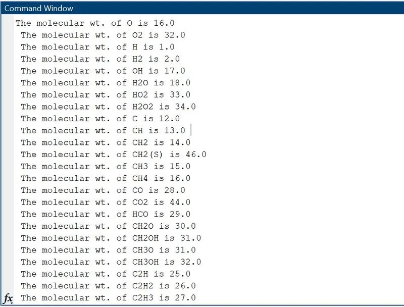
Molecular weight in command window values.
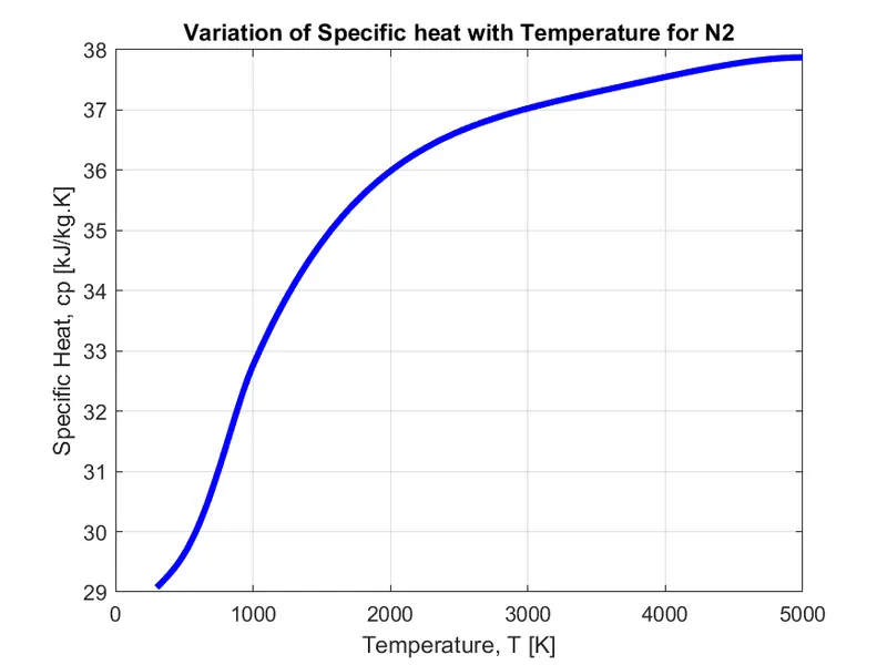
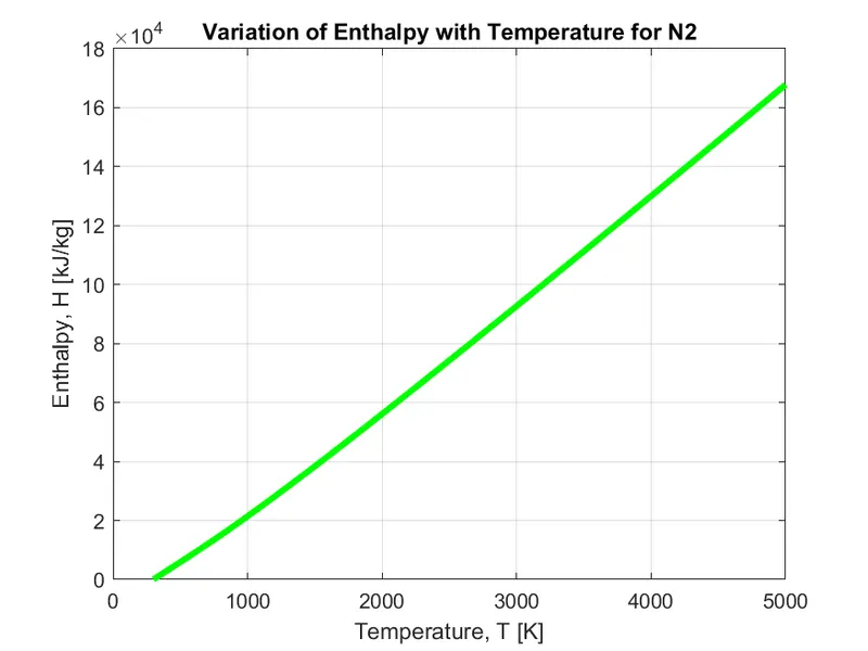
N2 output of Cp,H,S:
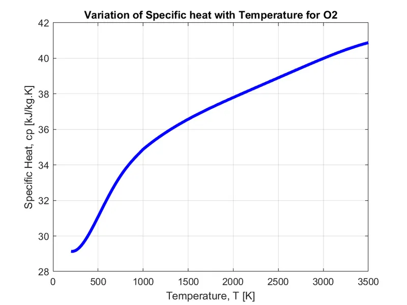
O2 output of Cp,H,S:
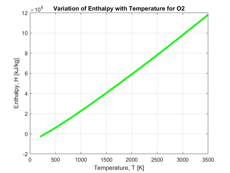
Output of Co2 in Cp,H,S:
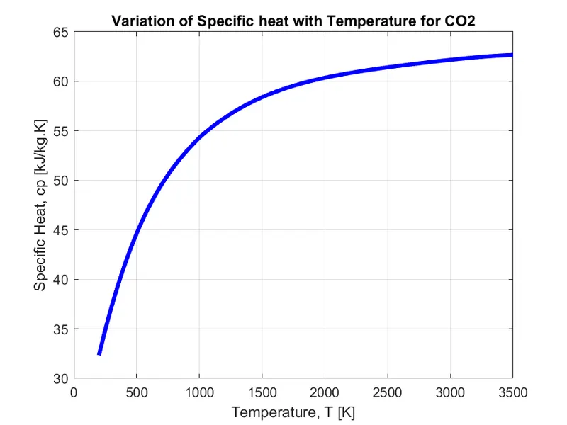
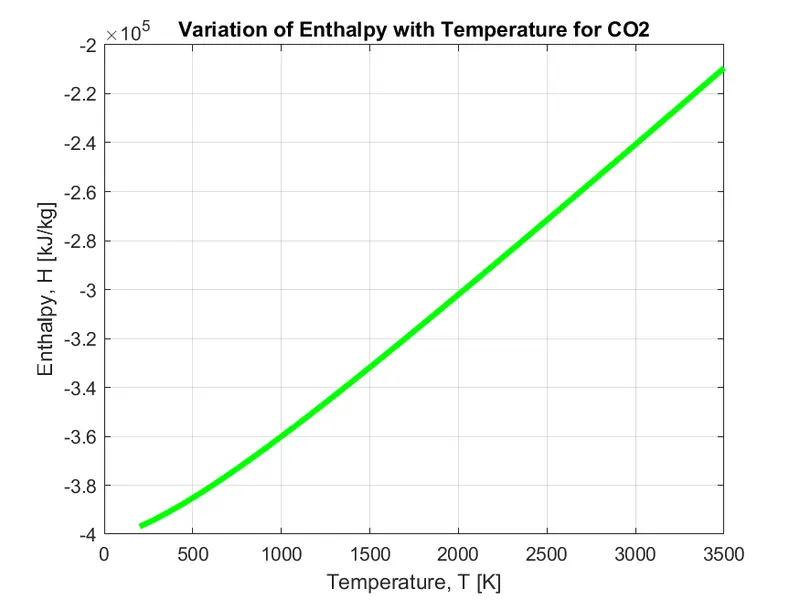
Preview of the folder in windows:

Error Occurs:
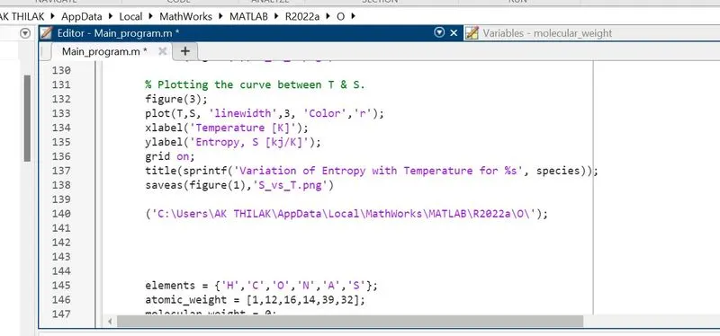
The error occurs because I forgot to include the Colon in Fig 2 and Fig 1 I forgot to include the cd code in the front of the directory and I include that program running fine.
References:
1. MATLAB Documentation strcmp
2. SkillLync Matlab Projects of NASA thermodynamic data